AJ_01_MPIL_Detection_and_Analysis_Tool

Author(s)

• Author1 = {“name”: “Anli Ji”, “affiliation”: “Department of Computer Science, Georgia State University, Atlanta, GA”, “email”: “aji1@student.gsu.edu”, “orcid”: “0000-0002-1551-2370”}

• Author2 = {“name”: “Nigar Khasayeva”, “affiliation”: “Department of Computer Science, Georgia State University, Atlanta, GA”, “email”: “nkhasayeva1@student.gsu.edu”, “orcid”: “0000-0002-4590-7031”}

• Author3 = {“name”: “Xumin Cai”, “affiliation”: “Department of Computer Science, Georgia State University, Atlanta, GA”, “email”: “xcai3@student.gsu.edu”, “orcid”: “”}

• Author4 = {“name”: “Manolis K. Georgoulis”, “affiliation”: “Research Center for Astronomy and Applied Mathematics, Academy of Athens, Greece”, “email”: “manolis.georgoulis@academyofathens.gr”, “orcid”: “0000-0001-6913-1330”}

• Author5 = {“name”: “Petrus C. Martens”, “affiliation”: “Department of Physics & Astronomy, Georgia State University, Atlanta, GA”, “email”: “martens@astro.gsu.edu”, “orcid”: “”}

• Author6 = {“name”: “Rafal A. Angryk”, “affiliation”: “Department of Computer Science, Georgia State University, Atlanta, GA”, “email”: “rangryk@cs.gsu.edu”, “orcid”: “0000-0001-9598-8207”}

• Author7 = {“name”: “Berkay Aydin”, “affiliation”: “Department of Computer Science, Georgia State University, Atlanta, GA”, “email”: “baydin2@gsu.edu”, “orcid”: “0000-0002-9799-9265”}

Table of Contents

• 1  MPIL_Detection_and_Analysis_Tool
  • 1.1  Author(s)
  • 1.2  Purpose
  • 1.3  Technical contributions
  • 1.4  Methodology
  • 1.5  Results
  • 1.6  Funding
  • 1.7  Keywords
  • 1.8  Citation
  • 1.9  Acknowledgements
• 2  Setup
  • 2.1  Library import
  • 2.2  Local library import
• 3  Parameter definitions
• 4  Data import
• 5  Detection process and analysis
  • 5.1  Identify Polarity Region by Strength threshold
  • 5.2  Apply Canny Edge Detection
  • 5.3  Extend the thickness of edge of Polarity region
  • 5.4  Candidate PIL
  • 5.5  Remove part based on magnetic field strength filter (95% threshold)
  • 5.6  Morphological thinning operations
  • 5.7  Further Filter PIL based on Length/Size (14 pixel)
  • 5.8  Generate Region of Polarity Inversions (RoPI)
  • 5.9  Generate convex hull of PIL
• 6  Video Analysis Tool
• 7  References

Purpose

Magnetic polarity inversion lines (MPILs) detected from solar active regions with attributes engineered from them are recognized as one of the essential features for predicting the characteristics of explosive and eruptive instabilities such as solar flares and coronal mass ejections (CME). We have built a software framework that can detect MPILs from the line-of-sight (LoS) or the radial component of the magnetic field vector in solar active region magnetogram patches. As part of our efforts, we applied this detection method on magnetogram patches obtained from HMI Active Region Patches (HARP) data product. This tool is customizable and can be used to detect, understand and analyze intrinsic characteristics of MPILs.

Technical contributions

• We share detection our tool in the notebook and present the inner works of our detection functions as well as visualization for the MPIL detection technique over a set of eruptive active regions from Solar Cycle 24.

• We also provide a qualitative evaluation of our module and exploratory analyses that highlight the relationships between the time evolution characteristics of MPILs in addition to a video visualization tool for the MPILs and related data products.

• The tools and code implemented in the notebook have been developed with user defined thresholds that allow easy modification for analysis.

Methodology

A brief summary of the detection method is as follows:

First, we identify the positive and negative polarity regions by applying a magnetic field strength threshold of +/-100 Gauss on active region magnetogram patches. Then, we obtain the boundaries of positive and negative polarity regions by using an edge detection technique and apply intersection and thinning morphological operations along with a magnetic field strength filter to identify coarse MPILs. Lastly, we generate final MPILs by imposing a size filter that removes the relatively small disconnected components/lines and retains more significant ones.

In addition to the MPIL detection tool, we provide feature extraction functions to obtain the properties of MPILs (i.e., MPIL size, the area of polarity inversion, the masked unsigned flux of enclosing MPIL, convexity, eigenvalues, fractal dimension, and Hu moments) and MPIL-related binary masks of rasters. These spatiotemporal data components can be extracted from any set of magnetogram patch series, which can be used to build a comprehensive and complementary data source for space weather forecasting efforts.

Results

This work provides a detection and visualization analysis tool for identifying MPILs and it can also be parameterized based on users’ requirements. We present detection results for a well-known active region, NOAA AR 11158 (HARP 377), consisting of 50 magnetogram patches (CEA series) with 1 hour cadence. Our detection results show that our approach can successfully identify PILs and other relevant metadata elements. Our video visualization tool can also be used to visually analyze the evolution of magnetic polarity inversion lines and their structure.

Funding

• Award = {“agency”: “NSF”, “award_code”: “2104004”, “award_URL”: “https://www.nsf.gov/awardsearch/showAward?AWD_ID=2104004”}

Keywords

keywords=[“Magnetic Polarity Inversion Lines”, “Solar Active Regions”, “Feature Extraction”]

Citation

A. Ji, N. Khasayeva, X. Cai, M. K. Georgoulis, P. C. Martens, R. A. Angryk, B. Aydin, 2022. MPIL Detection and Analysis Tool. Accessed 4/13/2022 at https://github.com/annieee6446/ec22-MPIL

Acknowledgements

The data used in this research is courtesy of NASA/SDO and the HMI science teams.

Setup

Library import

We will import glob for file operations. We will import sunpy.map and matplotlib.pylot for visualizations.

# File operations
import glob as glob
# Visualizations
import sunpy.map
import matplotlib.pyplot as plt

import warnings
warnings.filterwarnings('ignore')

Local library import

We will import the utility functions from our detection framework and video visualization tool.

# Include local library paths
import sys
sys.path.append('../utils')

# Import local libraries
from utils.region_detection import pos_neg_detection
from utils.pil_detection import detection
from utils.video_loading import video_loader

# Define HARP AR number as well as input and output path
HARP_AR = 377
input_path = './Sample_Input/'
output_path = './Sample_Output/'

# Create class object by initializing path to samples and the HARP number of the sample input
dt = pos_neg_detection()
pil_dt = detection(input_path,HARP_AR)
loader = video_loader()

# Check whether output path exists
pil_dt.check_outpath(output_path)

Parameter definitions

The tools and code implemented in the notebook have been developed with user defined thresholds that allow easy modification for analysis.

• STRENGTH_FILTER: Unsigned magnetic field strength threshold for identifying polarity regions.

• BUFFER_SIZE: Kernel size for spatial buffering of polarity region edges in pixels.

• PRESERVED_FLUX_RATIO: Flux threshold for filtering insignificant intersection regions based on accumulated flux. The minimum ratio of total unsigned flux to be preserved in polarity inversion regions is between [0, 1]

• MIN_MPIL_SIZE: Size filter threshold for removing small polarity inversion lines. It represents the minimum number of contiguous CEA pixels contained in each disconnected MPIL. Each pixel size from HARP series roughly covers 131,400 km^2.

STRENGTH_FILTER = 100
BUFFER_SIZE = 4
PRESERVED_FLUX_RATIO = 0.95
MIN_MPIL_SIZE = 14

Data import

Our PIL detection framework applies to longitudinal magnetogram patches. Throughout the development lifecycle of our framework, we made use of the HMI Active Region Patches (HARP) data product [1]. However, it can be used with other magnetogram data series. HARPs are essentially tracked active regions and come with both vector and LoS components of magnetic field. The LoS magnetic field product is stored in FITS format and can be accessed from JSOC (http://jsoc.stanford.edu/ajax/lookdata.html). We primarily used the definitive series with 720 seconds cadence which are mapped the Lambert Cylindrical Equal Area (CEA) projection, where each pixel roughly occupies the same physical area on the Sun. For brevity, in the samples shown below, we adopt a one hour cadence instead of the 720 seconds.

# Count the number of samples
data = glob.glob('./Sample_Input/377/*.fits')
print('Total number of sample images: ' + str(len(data)))

Total number of sample images: 50

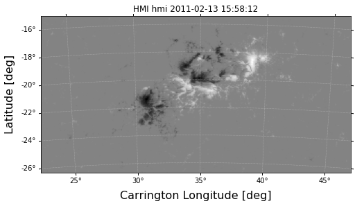
Plot out an example of imported data

# Specify the index of desired magnetogram patch
# Our sample includes 50 elements (indices 0 to 49)
data_index = 10

hmi_magmap = sunpy.map.Map(data[data_index])

fig = plt.figure(figsize=(8,6))
hmi_magmap.plot()
plt.xlabel('Carrington Longitude [deg]',fontsize = 16)
plt.ylabel('Latitude [deg]',fontsize = 16)
plt.show()

Detection process and analysis

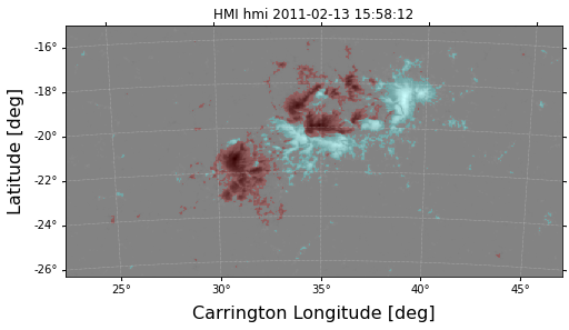
Identify Polarity Region by Strength threshold

The detection process starts by identifying the positive and negative polarity regions. We generated and applied two binary masks of the opposite polarity regions onto the original maps with a magnetic field strength thresholds of user defined Gauss values. The predefined thresholds are +/- 100 Gauss.

# Identify the positive and negative polarity regions
pos_377, neg_377 = dt.identify_pos_neg_region(hmi_magmap, pos_gauss = STRENGTH_FILTER, neg_gauss= -STRENGTH_FILTER)

# Create masks for the identified positive and negative polarity regions 
masked_pos = dt.mask_img(pos_377)
masked_neg = dt.mask_img(neg_377)

Light blue areas show the positive polarity regions

Dark red areas show negative polarity regions

fig = plt.figure(figsize=(8,6))
hmi_magmap.plot()
plt.imshow(masked_pos, 'cool', interpolation='none', alpha=0.2)
plt.imshow(masked_neg, 'autumn', interpolation='none', alpha=0.2)
plt.xlabel('Carrington Longitude [deg]',fontsize = 16)
plt.ylabel('Latitude [deg]',fontsize = 16)
plt.show()

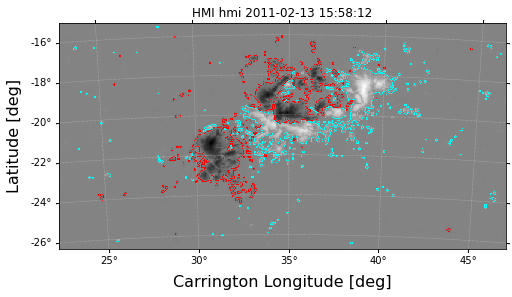
Apply Edge Detection

In this step, we obtain the boundaries of positive and negative polarity regions separately by using the Canny edge operator [2], which applies a Gaussian filter to smooth the magnetogram images and detects the overall contour of the polarity regions.

# Detect edges of the positive and negative polarity regions
pos_edge_377 = dt.edge_detection(pos_377)
neg_edge_377 = dt.edge_detection(neg_377)

# Create masks for the detected edges of positive and negative polarity regions
masked_pos_edge = dt.mask_img(pos_edge_377)
masked_neg_edge = dt.mask_img(neg_edge_377)

Light blue areas show the edges of positive polarity regions

Dark red areas show the edges of negative polarity regions

fig = plt.figure(figsize=(8,6))
hmi_magmap.plot()
plt.imshow(masked_pos_edge, 'cool', interpolation='none', alpha=1)
plt.imshow(masked_neg_edge, 'autumn', interpolation='none', alpha=1)
plt.xlabel('Carrington Longitude [deg]',fontsize = 16)
plt.ylabel('Latitude [deg]',fontsize = 16)
plt.show()

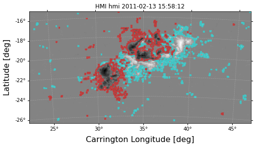
Apply spatial buffering on the edges of polarity regions

Region of Polarity Inversions (RoPIs) are the regions where negative and positive polarity regions are sufficiently close. These regions are determined using a topological intersection operation between spatially buffered edges of polarity regions. The intersection areas can then be considered as raw RoPIs. In this step, we spatially buffer the edges of negative and positive polarity regions in binary masks with a user defined buffer kernel size to represent the expanded areas of a given polarity inversion line. This buffer size parameter practically enforces how close polarity regions are expected to be located to be considered as adjacent regions.

# Spatially buffer edges of negative/positive polarity regions
pos_dil_edge_377 = dt.buff_edge(pos_edge_377, size = BUFFER_SIZE)
neg_dil_edge_377 = dt.buff_edge(neg_edge_377, size = BUFFER_SIZE)

# Create masks for the buffered edges
masked_pos_dil_edge = dt.mask_img(pos_dil_edge_377)
masked_neg_dil_edge = dt.mask_img(neg_dil_edge_377)

Light blue areas show the buffered edges of positive polarity regions

Dark red areas show the buffered edges of negative polarity regions

fig = plt.figure(figsize=(8,6))
hmi_magmap.plot()
plt.xlabel('Carrington Longitude [deg]',fontsize = 16)
plt.ylabel('Latitude [deg]',fontsize = 16)
plt.imshow(masked_pos_dil_edge, 'cool', interpolation='none', alpha=0.5)
plt.imshow(masked_neg_dil_edge, 'autumn', interpolation='none', alpha=0.5)
plt.show()

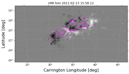
Candidate RoPIs

The candidate RoPIs are generated based on the intersection areas of spatially buffered opposite polarity regions.

In this step, we also include a quality index of SPEI (Severe Projection Effect Index) for checking magnetograms that can be potentially impacted by severe projection effect (greater than 70 degrees East-West).

pil_orig, label_orig = pil_dt.PIL_detect(pos_gauss = STRENGTH_FILTER, neg_gauss= -STRENGTH_FILTER, size_kernel = BUFFER_SIZE)

Number of Filtered Magnetograms after checking SPEI: 0
Number of Filtered Magnetograms after checking Patch Corner: 0
Number of Detected Candidate RoPIs:  50

# Generate index for matching the detected MPIL with the current sample
data_num = pil_dt.check_header(hmi_magmap)

# Create mask for detected MPIL
masked_pil = dt.mask_pil(label_orig[data_num])

fig = plt.figure(figsize=(8,6))
hmi_magmap.plot()
plt.imshow(masked_pil, 'spring', interpolation='none', alpha=1) # 'spring' represents the bright pink color
plt.xlabel('Carrington Longitude [deg]',fontsize = 16)
plt.ylabel('Latitude [deg]',fontsize = 16)
plt.show()

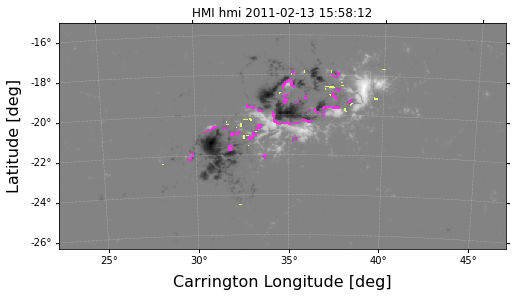
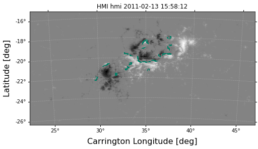
Candidate MPILs

Refine based on preserved flux ratio

To generate the candidate PILs, we utilize an unsigned magnetic flux filter on the areas covered by disconnected RoPIs, which ensures that the selected candidate PILs represent within the user defined percentage (denoted by PRESERVED_FLUX_RATIO) of unsigned magnetic flux contained in RoPIs and removes the candidate RoPIs with relatively low flux build up around them.

strength_label = pil_dt.filter_by_strength(threshold = PRESERVED_FLUX_RATIO)

masked_filter_RoPIs = dt.mask_pil(strength_label[data_num])

Magenda lines are the candidate MPILs

Light yellow parts are removed based on the filter threshold

fig = plt.figure(figsize=(8,6))
hmi_magmap.plot()
plt.imshow(masked_pil, 'Wistia', interpolation='none', alpha=1) # 'Wistia' represents the light yellow color
plt.imshow(masked_filter_RoPIs, 'spring', interpolation='none', alpha=0.8) # 'spring' represents the bright pink color
plt.xlabel('Carrington Longitude [deg]',fontsize = 16)
plt.ylabel('Latitude [deg]',fontsize = 16)
plt.show()

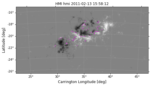
Morphological thinning operations

The flux filter is followed by applying a morphological thinning operation [3] to the candidate RoPIs. By doing this we eliminate majority of the foreground pixels and preserve the principal topology of the primary shapes for MPILs.

thin_df, thin_binary = pil_dt.thin_strength_label(strength_label)

masked_thinned_MPIL = dt.mask_pil(thin_binary[data_num])

fig = plt.figure(figsize=(8,6))
hmi_magmap.plot()
plt.imshow(masked_thinned_MPIL, 'spring', interpolation='none', alpha=1) # 'spring' represents the bright pink color
plt.xlabel('Carrington Longitude [deg]',fontsize = 12)
plt.ylabel('Latitude [deg]',fontsize = 12)
plt.show()

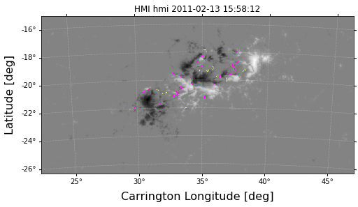
Further refinement using size filter

Lastly, we apply a user-defined size filter in CEA pixels. For HARP data series, each pixel roughly covers approximately 131,400 km^2. This operation removes relatively small MPILs and retain a cleaner set of significant MPILs. The predefined size is 14 pixels in this example.

filter_image = pil_dt.filter_by_size(thin_df, thin_binary, size_threshold = MIN_MPIL_SIZE)

masked_size_filter = dt.mask_pil(filter_image[data_num])

Magenda lines are the candidate MPILs

Light yellow parts are removed based on the filter threshold

fig = plt.figure(figsize=(8,6))
hmi_magmap.plot()
plt.imshow(masked_thinned_MPIL, 'Wistia', interpolation='none', alpha=1) # 'Wistia' represents the light yellow color
plt.imshow(masked_size_filter, 'spring', interpolation='none', alpha=1) # 'spring' represents the bright pink color
plt.xlabel('Carrington Longitude [deg]',fontsize = 16)
plt.ylabel('Latitude [deg]',fontsize = 16)
plt.show()

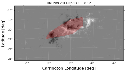
Getting Regions of Polarity Inversion (RoPI)

We fetch the refined RoPIs as part of our additional metadata raster.

ropi = pil_dt.RoPI(thin_df)

masked_ropi = dt.mask_pil(ropi[data_num])

fig = plt.figure(figsize=(8,6))
hmi_magmap.plot()
plt.imshow(masked_ropi, 'summer', interpolation='none', alpha=1) # 'summer' represents the green color
plt.xlabel('Carrington Longitude [deg]',fontsize = 16)
plt.ylabel('Latitude [deg]',fontsize = 16)
plt.show()

Getting convex hull of PIL

To generate the convex hull, we determine the convex closure of the set in detected MPIL.

convex_pil = pil_dt.convex_pil(filter_image)

masked_convex = dt.mask_pil(convex_pil[data_num])

fig = plt.figure(figsize=(8,6))
hmi_magmap.plot()
plt.imshow(masked_convex, 'autumn', interpolation='none', alpha=0.2)
plt.xlabel('Carrington Longitude [deg]',fontsize = 16)
plt.ylabel('Latitude [deg]',fontsize = 16)
plt.show()

Video Analysis Tool

Generates the magnetogram images of Active Regions with applied on them Polarity Inversion Line, Region of Polarity Inversion, and Convex Hull masks.

loader.build_images(input_path + str(HARP_AR), output_path + str(HARP_AR))

Displays the video slide of previously created magnetogram images.

video = loader.display_video(output_path + str(HARP_AR))
video

Reference

[1] M. G. Bobra, X. Sun, J. T. Hoeksema, M. Turmon, Y. Liu, K. Hayashi, G. Barnes, and K. D. Leka, “The helioseismic and magnetic imager (hmi) vector magnetic field pipeline: Sharps – space-weather hmi active region patches,” Solar Physics, vol. 289, no. 9, pp. 3549–3578, Sep 2014. Available: https://doi.org/10.1007/s11207-014-0529-3

[2] J. Canny, “A computational approach to edge detection,” IEEE Transactions on Pattern Analysis and Machine Intelligence, vol. PAMI-8, no. 6, pp. 679–698, 1986.

[3] Jean Serra. 1983. Image Analysis and Mathematical Morphology. Academic Press, Inc., USA.