ICESpark-EarthCube-2022-Annual-Meeting#

ICESpark in Action: Analyzing Large-scale Arctic Observations Using an Open-source Big Data Platform

Authors#

Author1 = {“name”: “Jia Yu”, “affiliation”: “Washington State University”, “email”: “jia.yu1@wsu.edu”}
Author2 = {“name”: “Yiqun Xie”, “affiliation”: “University of Maryland”, “email”: “xie@umd.edu”}
Author3 = {“name”: “Kyle Duncan”, “affiliation”: “University of Maryland”, “email”: “kduncan@umd.edu”}
Author4 = {“name”: “Sinead Louise Farrell”, “affiliation”: “University of Maryland”, “email”: “sineadf@umd.edu”}

Table of Contents#

ICESpark-EarthCube-2022-Annual-Meeting
Setup
Data import
Demo 1: Find the crossings between ICESat-2 orbits and SODA moorings
Demo 2: Find the crossing between ICESat-2 orbits and Sentinel-2 and WorldView-3 images
Demo 3: Find the crossings between ICESat-2 orbits and MOSAiC Master track of POLARSTERN cruise
References

Purpose#

The Arctic climate system is undergoing rapid change with rising air and sea surface temperatures, accompanied by declines in Arctic glacial ice and sea ice as well as loss of snow cover on land. The combined increase in global air temperature and ice-sheet mass loss is driving sea level rise around the globe. As the Arctic region is largely inaccessible to traditional observation techniques, satellite remote sensing systems play a key role in monitoring the essential climate variables. However, the unprecedented volume and variety of geospatial big data collected by new satellite sensors have reached far beyond the capacity of computing platforms accessible to most geoscientists. ICESpark is an open-source distributed platform that can combine local commodity computers into a powerful environment that is ready for geospatial big data (GeoBD). Built on Apache Sedona [1], ICESpark comprises a set of off-the-shelf data integration tools and analytical functions to make sense of large-scale arctic observations.

Technical contributions#

We plan to demonstrate ICESpark through a Python Jupyter notebook running on top of a cluster of commodity computers to let the audience experience the scalability and interactivity provided by the tool. In this notebook, we demonstrate three case studies to illustrate how ICESpark may help geoscientists quickly find temporally and/or spatially coincident data across heterogenous arctic observation data. This task is typically required to validate the accuracy of new remote sensing data products, or for cross comparison of complementary polar climate variables.

Results#

The first case study includes Stratified Ocean Dynamics of the Arctic (SODA) moorings [2] and ICESat-2 reference ground tracks (RGTs) [3], where the goal is to find all ICESat-2 orbits falling within a 50 km search radius around the mooring sites.
The second case study integrates Sentinel-2 [4] and WorldView-3 [5] imagery to discover the spatial overlaps between ICESat-2 RGTs and tiles from these high-resolution imagery datasets.
The last case study compares the aforementioned lCESat 2 orbits (RGTs) against the MOSAiC expedition cruise master track data [6 - 9]. The goal of this study is to find the spatio-temporal overalps between ICESat-Z orbits and a 50KM search radius around each reported cruise location.

Funding#

Award1 = {“agency”: “US National Science Foundation”, “award_code”: “2126449”, “award_URL”: “https://www.nsf.gov/awardsearch/showAward?AWD_ID=2126449&HistoricalAwards=false”}
Award2 = {“agency”: “US National Science Foundation”, “award_code”: “2126474”, “award_URL”: “https://www.nsf.gov/awardsearch/showAward?AWD_ID=2126474&HistoricalAwards=false”}

Keywords#

keywords=[“arctic observation”, “big data”, “cluster computing”]

Setup#

Library import#

## Import local library
import os
from datetime import datetime

## Import GeoPandas
import geopandas as gpd

## Import PySpark
from pyspark.sql import SparkSession
from pyspark.sql.types import *
from pyspark.sql.functions import col, expr, broadcast, udf

## Import Apache Sedona
from sedona.register import SedonaRegistrator
from sedona.utils import SedonaKryoRegistrator, KryoSerializer
from sedona.core.formatMapper.shapefileParser import ShapefileReader
from sedona.utils.adapter import Adapter

Initialize the cluster environment#

spark = SparkSession. \
    builder. \
    appName('appName'). \
    master('local[*]'). \
    config("spark.serializer", KryoSerializer.getName). \
    config("spark.kryo.registrator", SedonaKryoRegistrator.getName). \
    config('spark.jars.packages',
           'org.apache.sedona:sedona-python-adapter-3.0_2.12:1.2.0-incubating,org.datasyslab:geotools-wrapper:1.1.0-25.2'). \
    getOrCreate()

22/04/20 19:52:15 WARN Utils: Your hostname, jia-imac.local resolves to a loopback address: 127.0.0.1; using 10.71.12.51 instead (on interface en0)
22/04/20 19:52:15 WARN Utils: Set SPARK_LOCAL_IP if you need to bind to another address
WARNING: An illegal reflective access operation has occurred
WARNING: Illegal reflective access by org.apache.spark.unsafe.Platform (file:/Users/jiayu/.local/share/virtualenvs/gallery-icespark-yOC315wH/lib/python3.8/site-packages/pyspark/jars/spark-unsafe_2.12-3.1.2.jar) to constructor java.nio.DirectByteBuffer(long,int)
WARNING: Please consider reporting this to the maintainers of org.apache.spark.unsafe.Platform
WARNING: Use --illegal-access=warn to enable warnings of further illegal reflective access operations
WARNING: All illegal access operations will be denied in a future release

:: loading settings :: url = jar:file:/Users/jiayu/.local/share/virtualenvs/gallery-icespark-yOC315wH/lib/python3.8/site-packages/pyspark/jars/ivy-2.4.0.jar!/org/apache/ivy/core/settings/ivysettings.xml

Ivy Default Cache set to: /Users/jiayu/.ivy2/cache
The jars for the packages stored in: /Users/jiayu/.ivy2/jars
org.apache.sedona#sedona-python-adapter-3.0_2.12 added as a dependency
org.datasyslab#geotools-wrapper added as a dependency
:: resolving dependencies :: org.apache.spark#spark-submit-parent-22c315bb-e727-425e-b708-18068977ffae;1.0
	confs: [default]
	found org.apache.sedona#sedona-python-adapter-3.0_2.12;1.2.0-incubating in central
	found org.locationtech.jts#jts-core;1.18.0 in local-m2-cache
	found org.wololo#jts2geojson;0.16.1 in local-m2-cache
	found com.fasterxml.jackson.core#jackson-databind;2.12.2 in local-m2-cache
	found com.fasterxml.jackson.core#jackson-annotations;2.12.2 in local-m2-cache
	found com.fasterxml.jackson.core#jackson-core;2.12.2 in local-m2-cache
	found org.apache.sedona#sedona-core-3.0_2.12;1.2.0-incubating in local-m2-cache
	found org.scala-lang.modules#scala-collection-compat_2.12;2.5.0 in local-m2-cache
	found org.apache.sedona#sedona-sql-3.0_2.12;1.2.0-incubating in local-m2-cache
	found org.datasyslab#geotools-wrapper;1.1.0-25.2 in local-m2-cache
:: resolution report :: resolve 247ms :: artifacts dl 5ms
	:: modules in use:
	com.fasterxml.jackson.core#jackson-annotations;2.12.2 from local-m2-cache in [default]
	com.fasterxml.jackson.core#jackson-core;2.12.2 from local-m2-cache in [default]
	com.fasterxml.jackson.core#jackson-databind;2.12.2 from local-m2-cache in [default]
	org.apache.sedona#sedona-core-3.0_2.12;1.2.0-incubating from local-m2-cache in [default]
	org.apache.sedona#sedona-python-adapter-3.0_2.12;1.2.0-incubating from central in [default]
	org.apache.sedona#sedona-sql-3.0_2.12;1.2.0-incubating from local-m2-cache in [default]
	org.datasyslab#geotools-wrapper;1.1.0-25.2 from local-m2-cache in [default]
	org.locationtech.jts#jts-core;1.18.0 from local-m2-cache in [default]
	org.scala-lang.modules#scala-collection-compat_2.12;2.5.0 from local-m2-cache in [default]
	org.wololo#jts2geojson;0.16.1 from local-m2-cache in [default]
	:: evicted modules:
	org.locationtech.jts#jts-core;1.18.1 by [org.locationtech.jts#jts-core;1.18.0] in [default]
	---------------------------------------------------------------------
	|                  |            modules            ||   artifacts   |
	|       conf       | number| search|dwnlded|evicted|| number|dwnlded|
	---------------------------------------------------------------------
	|      default     |   11  |   0   |   0   |   1   ||   10  |   0   |
	---------------------------------------------------------------------
:: retrieving :: org.apache.spark#spark-submit-parent-22c315bb-e727-425e-b708-18068977ffae
	confs: [default]
	0 artifacts copied, 10 already retrieved (0kB/7ms)
22/04/20 19:52:16 WARN NativeCodeLoader: Unable to load native-hadoop library for your platform... using builtin-java classes where applicable
Using Spark's default log4j profile: org/apache/spark/log4j-defaults.properties
Setting default log level to "WARN".
To adjust logging level use sc.setLogLevel(newLevel). For SparkR, use setLogLevel(newLevel).

Register geospatial data support#

SedonaRegistrator.registerAll(spark)
sc = spark.sparkContext
sc.setSystemProperty("sedona.global.charset", "utf8")

[Stage 0:>                                                          (0 + 1) / 1]

                                                                                

Data import#

Load ICE_SAT2 orbits into Spark#

Files are originally in KML. They are converted to a single WKT file using GDAL ogr2ogr command.

The converted dataset contains 13704 orbits and has 2.6GB in size. The notebook only takes a sample of 499 orbits because of the limited resource provided in Binder environment. In addition, GitHub only allows max 100MB per file.

Filename example: IS2_RGT_0702_cycle3_14-May-2019.kml.csv

def orbit_date(s):
  length = len(s)
  date_str = s[(length-19):(length-8)]
  date_obj = datetime.strptime(date_str, '%d-%b-%Y')
#   return date_obj.strftime("%Y-%m-%d")
  return date_obj.strftime("%Y-%m")

# Add date UDF
spark.udf.register("orbit_date", orbit_date)

# Load data and create a Date column
spark.read.format("csv").\
    option("delimiter", ",").\
    option("header", "true").\
    load("data/IS2_RGTs_aggr_data_timestamp-head500.csv").\
    withColumn("date", expr("orbit_date(filename)")).\
    repartition(10).\
    createOrReplaceTempView("is2_df_raw")

Create DataFrame with a Geometry column#

spark.sql("select ST_FlipCoordinates(ST_GeomFromWKT(WKT)) as orbit, Name, altitudeMode, tessellate, extrude, visibility, filename, date from is2_df_raw").\
    createOrReplaceTempView("is2_df")

## Show the schema of the table
spark.table("is2_df").show(2)

## Show the names of the orbits
spark.table("is2_df").select("filename").show(10, truncate = False)

## Print the count. The total count should be 499
print(spark.table("is2_df").count())

+--------------------+-----+-------------+----------+-------+----------+--------------------+-------+
|               orbit| Name| altitudeMode|tessellate|extrude|visibility|            filename|   date|
+--------------------+-----+-------------+----------+-------+----------+--------------------+-------+
|LINESTRING (0.027...|RGT 1|clampToGround|        -1|      0|         1|IS2_RGT_0001_cycl...|2019-03|
|LINESTRING (0.027...|RGT 1|clampToGround|        -1|      0|         1|IS2_RGT_0001_cycl...|2020-06|
+--------------------+-----+-------------+----------+-------+----------+--------------------+-------+
only showing top 2 rows

+----------------------------------------+
|filename                                |
+----------------------------------------+
|IS2_RGT_0003_cycle10_24-Dec-2020.kml.csv|
|IS2_RGT_0003_cycle11_25-Mar-2021.kml.csv|
|IS2_RGT_0005_cycle2_28-Dec-2018.kml.csv |
|IS2_RGT_0005_cycle7_26-Mar-2020.kml.csv |
|IS2_RGT_0004_cycle2_28-Dec-2018.kml.csv |
|IS2_RGT_0006_cycle2_28-Dec-2018.kml.csv |
|IS2_RGT_0006_cycle5_27-Sep-2019.kml.csv |
|IS2_RGT_0006_cycle8_25-Jun-2020.kml.csv |
|IS2_RGT_0009_29-Dec-2018.kml.csv        |
|IS2_RGT_0010_29-Dec-2018.kml.csv        |
+----------------------------------------+
only showing top 10 rows

499

Read a country shapefile as the base map, for visualization purpose#

countries = ShapefileReader.readToGeometryRDD(sc, "data/ne_50m_admin_0_countries_lakes")
countries_df = Adapter.toDf(countries, spark).select("geometry", "NAME_EN")
countries_df.show(2)

22/04/20 19:52:24 WARN package: Truncated the string representation of a plan since it was too large. This behavior can be adjusted by setting 'spark.sql.debug.maxToStringFields'.

+--------------------+--------------------+
|            geometry|             NAME_EN|
+--------------------+--------------------+
|MULTIPOLYGON (((3...|Zimbabwe         ...|
|MULTIPOLYGON (((3...|Zambia           ...|
+--------------------+--------------------+
only showing top 2 rows

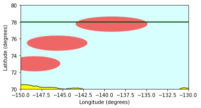
Demo 1: Find the crossings between ICESat-2 orbits and SODA moorings#

We have 3 Stratified Ocean Dynamics of the Arctic (SODA) moorings sites at the following locations:

SODA-A: (73.00043, -148.33627)

SODA-B: (75.46388, -145.63685)

SODA-C: (77.73677, -139.14153)

Find the crossings around three SODA objects, each of which has a 100KM buffer area, using ST_Buffer#

IceSat2 data needs to be converted from WGS84 (epsg:4326) CRS to meter-based epsg:4087 (WGS 84 / World Equidistant Cylindrical) using Sedona’s ST_Transform

result_df1 = spark.sql('SELECT * '
                     'FROM is2_df '
                     'WHERE ST_Intersects(ST_Buffer(ST_Transform(ST_POINT (73.00043,-148.33627), \'epsg:4326\',\'epsg:4087\'), 100000), ST_Transform(orbit, \'epsg:4326\',\'epsg:4087\'))')
result_df1.show(2)
print('SODA-A crosses: ', result_df1.count())

result_df2 = spark.sql('SELECT * '
                     'FROM is2_df '
                     'WHERE ST_Intersects(ST_Buffer(ST_Transform(ST_POINT (75.46388,-145.63685), \'epsg:4326\',\'epsg:4087\'), 100000), ST_Transform(orbit, \'epsg:4326\',\'epsg:4087\'))')
print('SODA-B crosses: ', result_df2.count())

result_df3 = spark.sql('SELECT * '
                     'FROM is2_df '
                     'WHERE ST_Intersects(ST_Buffer(ST_Transform(ST_POINT (77.73677, -139.14153), \'epsg:4326\',\'epsg:4087\'), 100000), ST_Transform(orbit, \'epsg:4326\',\'epsg:4087\'))')
print('SODA-C crosses: ', result_df3.count())

+--------------------+------+-------------+----------+-------+----------+--------------------+-------+
|               orbit|  Name| altitudeMode|tessellate|extrude|visibility|            filename|   date|
+--------------------+------+-------------+----------+-------+----------+--------------------+-------+
|LINESTRING (0.025...|RGT 22|clampToGround|        -1|      0|         1|IS2_RGT_0022_cycl...|2020-03|
|LINESTRING (0.025...|RGT 22|clampToGround|        -1|      0|         1|IS2_RGT_0022_cycl...|2020-09|
+--------------------+------+-------------+----------+-------+----------+--------------------+-------+
only showing top 2 rows

SODA-A crosses:  10

SODA-B crosses:  0

[Stage 23:==>                                                     (1 + 19) / 20]

SODA-C crosses:  10

[Stage 23:================>                                       (6 + 14) / 20]

                                                                                

Find orbits in Year 2019 in the SODA-C result#

result_df3_sorted = result_df3.filter("filename LIKE \'%2019%\'").sort(col('filename').asc())
result_df3_sorted.select('filename').show(truncate = False)

+---------------------------------------+
|filename                               |
+---------------------------------------+
|IS2_RGT_0008_cycle3_29-Mar-2019.kml.csv|
|IS2_RGT_0008_cycle5_27-Sep-2019.kml.csv|
|IS2_RGT_0008_cycle6_27-Dec-2019.kml.csv|
+---------------------------------------+

Visualize crossings on SODA-C using GeoPandas#

Put SODA-C into a DF and convert it to 100KM circle#

soda_list = ["POINT (73.00043 -148.33627)", "POINT (75.46388 -145.63685)", "POINT (77.73677 -139.14153)"]
# soda_list = ["POINT (77.73677 -139.14153)"]
soda_df = spark.createDataFrame(soda_list,StringType())
# Convert to epsg:4087 meter-based CRS
soda_df = soda_df.selectExpr('ST_Transform(ST_GeomFromWKT(value), \'epsg:4326\',\'epsg:3413\') as is2_df')
soda_df.show()
# Create circles using 50KM
soda_df = soda_df.selectExpr('ST_Buffer(is2_df, 100000) as is2_df')
# Convert to epsg:4326 WGS84
soda_df = soda_df.selectExpr('ST_FlipCoordinates(ST_Transform(is2_df, \'epsg:3413\',\'epsg:4326\')) as is2_df')
# soda_df.show()

+--------------------+
|              is2_df|
+--------------------+
|POINT (-1804587.9...|
|POINT (-1555620.5...|
|POINT (-1329850.8...|
+--------------------+

Convert SODA-C result DataFrame to GeoPandas DataFrame#

country_gpd = gpd.GeoDataFrame(countries_df.toPandas(), geometry="geometry")
soda_gpd = gpd.GeoDataFrame(soda_df.toPandas(), geometry="is2_df")
orbit_gpd = gpd.GeoDataFrame(result_df3.selectExpr('ST_FlipCoordinates(orbit) as orbit').toPandas(), geometry="orbit")

/Users/jiayu/.local/share/virtualenvs/gallery-icespark-yOC315wH/lib/python3.8/site-packages/geopandas/array.py:85: ShapelyDeprecationWarning: __len__ for multi-part geometries is deprecated and will be removed in Shapely 2.0. Check the length of the `geoms` property instead to get the  number of parts of a multi-part geometry.
  aout[:] = out
/Users/jiayu/.local/share/virtualenvs/gallery-icespark-yOC315wH/lib/python3.8/site-packages/geopandas/geodataframe.py:35: ShapelyDeprecationWarning: The array interface is deprecated and will no longer work in Shapely 2.0. Convert the '.coords' to a numpy array instead.
  out = from_shapely(data)

Plot the maps#

You can uncomment different base XY to change the view of the map

base = country_gpd.plot(color='yellow', edgecolor='black', zorder=1)
base.set_facecolor('#d7fffe')
# SODA-A Close-up view
#base.set_xlim(-151, -146)
#base.set_ylim(71, 75)
# SODA-B Close-up view
#base.set_xlim(-147.5, -143.5)
#base.set_ylim(74, 77)
# SODA-C Close-up view
base.set_xlim(-150, -130)
base.set_ylim(70, 80)
# SODA-ABC Close-up view
# base.set_xlim(-160, -130)
# base.set_ylim(60, 90)
# Global view
# base.set_xlim(-180, 180)
# base.set_ylim(-90, 90)
base.set_xlabel('Longitude (degrees)')
base.set_ylabel('Latitude (degrees)')
orbit = orbit_gpd.plot(ax=base, color='#06470c', zorder=3)
soda = soda_gpd.plot(ax=orbit, color='red', alpha=0.6, zorder=2)

/Users/jiayu/.local/share/virtualenvs/gallery-icespark-yOC315wH/lib/python3.8/site-packages/geopandas/plotting.py:38: ShapelyDeprecationWarning: Iteration over multi-part geometries is deprecated and will be removed in Shapely 2.0. Use the `geoms` property to access the constituent parts of a multi-part geometry.
  for poly in geom:
/Users/jiayu/.local/share/virtualenvs/gallery-icespark-yOC315wH/lib/python3.8/site-packages/descartes/patch.py:62: ShapelyDeprecationWarning: The array interface is deprecated and will no longer work in Shapely 2.0. Convert the '.coords' to a numpy array instead.
  vertices = concatenate([
/Users/jiayu/.local/share/virtualenvs/gallery-icespark-yOC315wH/lib/python3.8/site-packages/descartes/patch.py:64: ShapelyDeprecationWarning: The array interface is deprecated and will no longer work in Shapely 2.0. Convert the '.coords' to a numpy array instead.
  [asarray(r)[:, :2] for r in t.interiors])
/Users/jiayu/.local/share/virtualenvs/gallery-icespark-yOC315wH/lib/python3.8/site-packages/geopandas/plotting.py:171: ShapelyDeprecationWarning: The array interface is deprecated and will no longer work in Shapely 2.0. Convert the '.coords' to a numpy array instead.
  segments = [np.array(linestring)[:, :2] for linestring in geoms]
/Users/jiayu/.local/share/virtualenvs/gallery-icespark-yOC315wH/lib/python3.8/site-packages/descartes/patch.py:62: ShapelyDeprecationWarning: The array interface is deprecated and will no longer work in Shapely 2.0. Convert the '.coords' to a numpy array instead.
  vertices = concatenate([

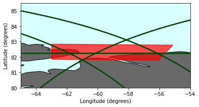
../../_images/ICESpark-EarthCube-2022-Annual-Meeting_26_1.png

Demo 2: Find the crossing between ICESat-2 orbits and Sentinel-2 and WorldView-3 images#

Two Sentinel-2 image bounding boxes (lat, lon format)

S-2 image from June 22, 2019:

UL: 82.852919, -63.001439
LL: 81.869306, -63.001267
UR: 82.785942, -55.145842
LR: 81.810456, -56.080844

Polygon format (UL - LL - LR - UR - UL): 82.852919, -63.001439, 81.869306, -63.001267, 81.810456, -56.080844, 82.785942, -55.145842, 82.852919, -63.001439

S-2 image from September 3, 2019:

UL: 79.232286, -121.801758
LL: 78.251639, -121.405181
UR: 79.268856, -116.530467
LR: 78.285072, -116.569403

Polygon format (UL - LL - LR - UR - UL): 79.232286, -121.801758, 78.251639, -121.405181, 78.285072, -116.569403, 79.268856, -116.530467, 79.232286, -121.801758

WorldView image bounding boxes (lat, lon format)

WV-3 image from April 10, 2019

UL: 79.76066207, -114.09955772
LL: 79.62275657, -114.06853064
UR: 79.83858880, -112.31487793
LR: 79.69303180, -112.34933739

Polygon format (UL - LL - LR - UR - UL): 79.76066207, -114.09955772, 79.62275657, -114.06853064, 79.69303180, -112.34933739, 79.83858880, -112.31487793, 79.76066207, -114.09955772

WV-2 image from April 10, 2019

UL: 80.0576610499, -110.56248745
LL: 79.9244458799, -110.56242819
UR: 80.044587680, -109.42456569
LR: 79.9092631399, -109.42423191

Polygon format (UL - LL - LR - UR - UL): 80.0576610499, -110.56248745, 79.9244458799, -110.56242819, 79.9092631399, -109.42423191, 80.044587680, -109.42456569, 80.0576610499, -110.56248745

WV-2 image from June 25, 2020

UL: 84.04474275, -60.80835633
LL: 83.90936693, -60.7855143
UR: 84.04404486, -59.21133579
LR: 83.90966186, -59.23332056

Polygon format (UL - LL - LR - UR - UL): 84.04474275, -60.80835633, 83.90936693, -60.7855143, 83.90966186, -59.23332056, 84.04404486, -59.21133579, 84.04474275, -60.80835633

Check if orbits intersect S-2 and/or WorldView bounding boxes#

# modified projection

result_df1 = spark.sql('SELECT * '
                     'FROM is2_df '
                     'WHERE ST_Intersects(orbit, ST_PolygonFromText (\'82.852919, -63.001439,81.869306, -63.001267, 81.810456, -56.080844, 82.785942, -55.145842, 82.852919, -63.001439\',\',\'))')
result_df1.select("filename").show(truncate = False)
print('Sentinel-2 A number of crosses: ', result_df1.count())

result_df2 = spark.sql('SELECT * '
                     'FROM is2_df '
                     'WHERE ST_Intersects(orbit, ST_PolygonFromText (\'79.232286, -121.801758, 78.251639, -121.405181, 78.285072, -116.569403, 79.268856, -116.530467, 79.232286, -121.801758\',\',\'))')
print('Sentinel-2 B number of crosses: ', result_df2.count())

result_df3 = spark.sql('SELECT * '
                      'FROM is2_df '
                      'WHERE ST_Intersects(orbit, ST_PolygonFromText (\'79.76066207, -114.09955772, 79.62275657, -114.06853064, 79.69303180, -112.34933739, 79.83858880, -112.31487793, 79.76066207, -114.09955772\',\',\'))')
print('WorldView A number of crosses: ', result_df3.count())

result_df4 = spark.sql('SELECT * '
                     'FROM is2_df '
                     'WHERE ST_Intersects(orbit, ST_PolygonFromText (\'80.0576610499, -110.56248745, 79.9244458799, -110.56242819, 79.9092631399, -109.42423191, 80.044587680, -109.42456569, 80.0576610499, -110.56248745\',\',\'))')
print('WorldView B number of crosses: ', result_df4.count())

result_df5 = spark.sql('SELECT * '
                     'FROM is2_df '
                     'WHERE ST_Intersects(orbit, ST_PolygonFromText (\'84.04474275, -60.80835633, 83.90936693, -60.7855143, 83.90966186, -59.23332056, 84.04404486, -59.21133579, 84.04474275, -60.80835633\',\',\'))')
print('WorldView C number of crosses: ', result_df5.count())

[Stage 35:==>                                                     (1 + 19) / 20]

                                                                                

+----------------------------------------+
|filename                                |
+----------------------------------------+
|IS2_RGT_0018_cycle2_29-Dec-2018.kml.csv |
|IS2_RGT_0023_cycle11_26-Mar-2021.kml.csv|
|IS2_RGT_0033_30-Dec-2018.kml.csv        |
|IS2_RGT_0018_cycle7_27-Mar-2020.kml.csv |
|IS2_RGT_0023_cycle3_30-Mar-2019.kml.csv |
|IS2_RGT_0033_cycle8_27-Jun-2020.kml.csv |
|IS2_RGT_0018_cycle6_27-Dec-2019.kml.csv |
|IS2_RGT_0023_cycle9_25-Sep-2020.kml.csv |
|IS2_RGT_0033_cycle6_28-Dec-2019.kml.csv |
|IS2_RGT_0042_cycle3_01-Apr-2019.kml.csv |
|IS2_RGT_0042_cycle7_29-Mar-2020.kml.csv |
|IS2_RGT_0018_cycle11_25-Mar-2021.kml.csv|
|IS2_RGT_0023_cycle10_25-Dec-2020.kml.csv|
|IS2_RGT_0033_cycle2_30-Dec-2018.kml.csv |
|IS2_RGT_0042_cycle11_27-Mar-2021.kml.csv|
|IS2_RGT_0042_cycle8_28-Jun-2020.kml.csv |
|IS2_RGT_0018_cycle8_26-Jun-2020.kml.csv |
|IS2_RGT_0023_cycle2_29-Dec-2018.kml.csv |
|IS2_RGT_0033_cycle7_28-Mar-2020.kml.csv |
|IS2_RGT_0042_31-Dec-2018.kml.csv        |
+----------------------------------------+
only showing top 20 rows

Sentinel-2 A number of crosses:  40

[Stage 42:===============================================>        (17 + 3) / 20]

                                                                                

Sentinel-2 B number of crosses:  10

[Stage 45:==>                                                     (1 + 19) / 20]

                                                                                

WorldView A number of crosses:  0
WorldView B number of crosses:  0
WorldView C number of crosses:  10

Find orbits in Year 2019 in the S-2 A result#

result_df1.filter('filename LIKE \'%2019%\'').select("filename").show(result_df1.count(), truncate = False)

[Stage 54:==================================================>     (18 + 2) / 20]

                                                                                

+---------------------------------------+
|filename                               |
+---------------------------------------+
|IS2_RGT_0018_cycle6_27-Dec-2019.kml.csv|
|IS2_RGT_0042_cycle3_01-Apr-2019.kml.csv|
|IS2_RGT_0018_cycle5_28-Sep-2019.kml.csv|
|IS2_RGT_0042_cycle6_29-Dec-2019.kml.csv|
|IS2_RGT_0018_cycle3_30-Mar-2019.kml.csv|
|IS2_RGT_0042_cycle5_29-Sep-2019.kml.csv|
|IS2_RGT_0023_cycle6_28-Dec-2019.kml.csv|
|IS2_RGT_0023_cycle5_28-Sep-2019.kml.csv|
|IS2_RGT_0023_cycle3_30-Mar-2019.kml.csv|
|IS2_RGT_0033_cycle3_31-Mar-2019.kml.csv|
|IS2_RGT_0033_cycle6_28-Dec-2019.kml.csv|
|IS2_RGT_0033_cycle5_29-Sep-2019.kml.csv|
+---------------------------------------+

Visualize crossings on S-2 A using GeoPandas#

Put S-2 A into a DataFrame#

You can uncomment other examples as well

s2_a = spark.sql('SELECT ST_FlipCoordinates(ST_PolygonFromText (\'82.852919, -63.001439, 81.869306, -63.001267, 81.810456, -56.080844, 82.785942, -55.145842, 82.852919, -63.001439\',\',\')) as s2a')
s2_a.show()
#s2_a = spark.sql('SELECT ST_FlipCoordinates(ST_PolygonFromText (\'82.852919, -63.001439, 81.869306, -63.001267, 81.810456, -56.080844, 82.785942, -55.145842, 82.852919, -63.001439\',\',\')) as s2a')
#s2_b = spark.sql('SELECT ST_FlipCoordinates(ST_PolygonFromText (\'79.232286, -121.801758, 78.251639, -121.405181, 78.285072, -116.569403, 79.268856, -116.530467, 79.232286, -121.801758\',\',\')) as s2b')
# wv_a = spark.sql('SELECT ST_FlipCoordinates(ST_PolygonFromText (\'79.76066207, -114.09955772, 79.62275657, -114.06853064, 79.69303180, -112.34933739, 79.83858880, -112.31487793, 79.76066207, -114.09955772\',\',\')) as wva')
#s2_a.show()
#s2_b.show()
#wv_a.show()

+--------------------+
|                 s2a|
+--------------------+
|POLYGON ((-63.001...|
+--------------------+

Convert result DataFrame to GeoPandas DataFrame#

country_gpd = gpd.GeoDataFrame(countries_df.toPandas(), geometry="geometry")
## Separate lines for each example
s2_gpd = gpd.GeoDataFrame(s2_a.toPandas(), geometry="s2a")
#s2_gpd = gpd.GeoDataFrame(s2_b.toPandas(), geometry="s2b")
# wv_gpd = gpd.GeoDataFrame(wv_a.toPandas(), geometry="wva")
orbit_gpd = gpd.GeoDataFrame(result_df1.selectExpr('ST_FlipCoordinates(orbit) as orbit').toPandas(), geometry="orbit")
#orbit_gpd = gpd.GeoDataFrame(result_df2.selectExpr('ST_FlipCoordinates(orbit) as orbit').toPandas(), geometry="orbit")
# orbit_gpd = gpd.GeoDataFrame(result_df3.selectExpr('ST_FlipCoordinates(orbit) as orbit').toPandas(), geometry="orbit")

/Users/jiayu/.local/share/virtualenvs/gallery-icespark-yOC315wH/lib/python3.8/site-packages/geopandas/array.py:85: ShapelyDeprecationWarning: __len__ for multi-part geometries is deprecated and will be removed in Shapely 2.0. Check the length of the `geoms` property instead to get the  number of parts of a multi-part geometry.
  aout[:] = out
/Users/jiayu/.local/share/virtualenvs/gallery-icespark-yOC315wH/lib/python3.8/site-packages/geopandas/geodataframe.py:35: ShapelyDeprecationWarning: The array interface is deprecated and will no longer work in Shapely 2.0. Convert the '.coords' to a numpy array instead.
  out = from_shapely(data)

Plot the maps#

You can uncomment different base XY to change the view of the map

base = country_gpd.plot(color='dimgray', edgecolor='black', zorder=1)
base.set_facecolor('#d7fffe')
# Sentinel-2 A view
base.set_xlim(-65, -54)
base.set_ylim(80, 85.5)
# Sentinel-2 B view
#base.set_xlim(-125, -113)
#base.set_ylim(72, 80)
# WorldView A view
# base.set_xlim(-115, -111)
# base.set_ylim(78, 81)
# Global view
#base.set_xlim(-180, 180)
#base.set_ylim(-90, 90)
base.set_xlabel('Longitude (degrees)')
base.set_ylabel('Latitude (degrees)')
orbit = orbit_gpd.plot(ax=base, color='#06470c', linewidth=1.75, label='IS2 RGT 1298 & 1307', zorder=3)
s2 = s2_gpd.plot(ax=orbit, color='red', alpha=0.7, edgecolor='red', linewidth=1.75, zorder=2)
# wv = wv_gpd.plot(ax=orbit, color='red', alpha=0.7, edgecolor='red', linewidth=1.75, label='WV-2 Image', zorder=2)
#plt.legend(loc='upper right', framealpha=1)
#plt.title('June 22, 2019 Sentinel-2 and IS-2 crossing')
#plt.show()

/Users/jiayu/.local/share/virtualenvs/gallery-icespark-yOC315wH/lib/python3.8/site-packages/geopandas/plotting.py:38: ShapelyDeprecationWarning: Iteration over multi-part geometries is deprecated and will be removed in Shapely 2.0. Use the `geoms` property to access the constituent parts of a multi-part geometry.
  for poly in geom:
/Users/jiayu/.local/share/virtualenvs/gallery-icespark-yOC315wH/lib/python3.8/site-packages/descartes/patch.py:62: ShapelyDeprecationWarning: The array interface is deprecated and will no longer work in Shapely 2.0. Convert the '.coords' to a numpy array instead.
  vertices = concatenate([
/Users/jiayu/.local/share/virtualenvs/gallery-icespark-yOC315wH/lib/python3.8/site-packages/descartes/patch.py:64: ShapelyDeprecationWarning: The array interface is deprecated and will no longer work in Shapely 2.0. Convert the '.coords' to a numpy array instead.
  [asarray(r)[:, :2] for r in t.interiors])
/Users/jiayu/.local/share/virtualenvs/gallery-icespark-yOC315wH/lib/python3.8/site-packages/geopandas/plotting.py:171: ShapelyDeprecationWarning: The array interface is deprecated and will no longer work in Shapely 2.0. Convert the '.coords' to a numpy array instead.
  segments = [np.array(linestring)[:, :2] for linestring in geoms]
/Users/jiayu/.local/share/virtualenvs/gallery-icespark-yOC315wH/lib/python3.8/site-packages/descartes/patch.py:62: ShapelyDeprecationWarning: The array interface is deprecated and will no longer work in Shapely 2.0. Convert the '.coords' to a numpy array instead.
  vertices = concatenate([

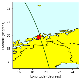
../../_images/ICESpark-EarthCube-2022-Annual-Meeting_38_1.png

Demo 3: Find the crossings between ICESat-2 orbits and MOSAiC Master track of POLARSTERN cruise#

# Create a UDF to clean up the data
def cruise_date(s):
#   return s[0:10]
  return s[0:7]
spark.udf.register("cruise_date", cruise_date)

<function __main__.cruise_date(s)>

Load Master track of POLARSTERN cruise into Spark#

The original data contains Leg 1- 4 including 28222065 coordinates, and has a size at 1.2 GB

This demo only takes a sample of 1000 records.

cruise_df = spark.read.format("csv").\
    option("delimiter", "\t").\
    option("header", "true").\
    load("data/PS122*head1000.txt").\
    filter(col("Latitude").isNotNull()).\
    filter(col("Longitude").isNotNull()).\
    repartition(10)
cruise_df.show(2)

+-------------------+----------+----------+--------------------+
|    Date/Time (UTC)|  Latitude| Longitude|Flag for data source|
+-------------------+----------+----------+--------------------+
|2019-09-20T17:30:03|69.6795466|18.9966542|                   2|
|2019-09-20T17:44:29|69.6795462|18.9966490|                   2|
+-------------------+----------+----------+--------------------+
only showing top 2 rows

Create a DataFrame with a Geometry column#

cruise_df = cruise_df.withColumn("location", expr("ST_Point(cast(Longitude as double), cast(Latitude as double))"))\
.drop("Longitude").drop("Latitude").withColumn("date", expr("cruise_date(`Date/Time (UTC)`)"))
# .filter("`Date/Time (UTC)` LIKE \'2020______T__:00:00\'")
# cruise_df.createOrReplaceTempView("cruise_df")
cruise_df.show(2)
cruise_df.select("location").show(2, truncate = False)
print(cruise_df.count())

+-------------------+--------------------+--------------------+-------+
|    Date/Time (UTC)|Flag for data source|            location|   date|
+-------------------+--------------------+--------------------+-------+
|2019-09-20T17:30:03|                   2|POINT (18.9966542...|2019-09|
|2019-09-20T17:44:29|                   2|POINT (18.996649 ...|2019-09|
+-------------------+--------------------+--------------------+-------+
only showing top 2 rows

+-----------------------------+
|location                     |
+-----------------------------+
|POINT (18.9966479 69.6795465)|
|POINT (18.9966463 69.6795468)|
+-----------------------------+
only showing top 2 rows

999

Find orbits within a 50KM circle of cruise locations in Year 2019, using ST_Buffer#

IceSat2 data needs to be converted from WGS84 (epsg:4326) CRS to meter-based epsg:4087 (WGS 84 / World Equidistant Cylindrical) using Sedona’s ST_Transform

result_df = cruise_df.join(spark.table("is2_df").filter('filename LIKE \'%2019%\'').select("orbit", "date"), 'date').\
    filter("ST_Intersects(ST_Transform(ST_Buffer(ST_Transform(location, \'epsg:4326\',\'epsg:3413\'), 50000), \'epsg:3413\',\'epsg:4326\'), ST_FlipCoordinates(orbit))").\
    cache()
print('The number of crossings pairs: ', result_df.count())
result_df = result_df.limit(1000) # Only send 1000 rows for visualization
result_df.show(10)

22/04/20 19:52:42 WARN JoinQuery: UseIndex is true, but no index exists. Will build index on the fly.
                                                                                

The number of crossings pairs:  999
+-------+-------------------+--------------------+--------------------+--------------------+
|   date|    Date/Time (UTC)|Flag for data source|            location|               orbit|
+-------+-------------------+--------------------+--------------------+--------------------+
|2019-09|2019-09-20T17:41:16|                   2|POINT (18.9966465...|LINESTRING (-0.00...|
|2019-09|2019-09-20T17:34:21|                   2|POINT (18.9966453...|LINESTRING (-0.00...|
|2019-09|2019-09-20T17:40:45|                   2|POINT (18.9966464...|LINESTRING (-0.00...|
|2019-09|2019-09-20T17:41:11|                   2|POINT (18.9966465...|LINESTRING (-0.00...|
|2019-09|2019-09-20T17:40:50|                   2|POINT (18.9966464...|LINESTRING (-0.00...|
|2019-09|2019-09-20T17:41:15|                   2|POINT (18.9966465...|LINESTRING (-0.00...|
|2019-09|2019-09-20T17:40:37|                   2|POINT (18.9966463...|LINESTRING (-0.00...|
|2019-09|2019-09-20T17:41:14|                   2|POINT (18.9966465...|LINESTRING (-0.00...|
|2019-09|2019-09-20T17:40:57|                   2|POINT (18.9966465...|LINESTRING (-0.00...|
|2019-09|2019-09-20T17:41:17|                   2|POINT (18.9966465...|LINESTRING (-0.00...|
+-------+-------------------+--------------------+--------------------+--------------------+
only showing top 10 rows

Visualize the query result using GeoPandas#

Convert Cruise DF to 50KM circle#

# Convert to epsg:4087 meter-based CRS
# Only send 1000 locations for visualization
cruise_df_viz = result_df.selectExpr('ST_Transform(location, \'epsg:4326\',\'epsg:3413\') as location')
# cruise_df.show()
# # Create circles using 50KM
cruise_df_viz = cruise_df_viz.selectExpr('ST_Buffer(location, 50000) as location')
# # Convert to epsg:4326 WGS84
cruise_df_viz = cruise_df_viz.selectExpr('ST_Transform(location, \'epsg:3413\',\'epsg:4326\') as location')
cruise_df_viz.show(10)

+--------------------+
|            location|
+--------------------+
|POLYGON ((18.7160...|
|POLYGON ((18.7160...|
|POLYGON ((18.7160...|
|POLYGON ((18.7160...|
|POLYGON ((18.7160...|
|POLYGON ((18.7160...|
|POLYGON ((18.7160...|
|POLYGON ((18.7160...|
|POLYGON ((18.7160...|
|POLYGON ((18.7160...|
+--------------------+
only showing top 10 rows

Convert to GeoPandas DataFrames#

country_gpd = gpd.GeoDataFrame(countries_df.toPandas(), geometry="geometry")
cruise_gpd = gpd.GeoDataFrame(cruise_df_viz.toPandas(), geometry="location")
orbit_gpd = gpd.GeoDataFrame(result_df.selectExpr('ST_FlipCoordinates(orbit) as orbit').distinct().toPandas(), geometry="orbit")

/Users/jiayu/.local/share/virtualenvs/gallery-icespark-yOC315wH/lib/python3.8/site-packages/geopandas/array.py:85: ShapelyDeprecationWarning: __len__ for multi-part geometries is deprecated and will be removed in Shapely 2.0. Check the length of the `geoms` property instead to get the  number of parts of a multi-part geometry.
  aout[:] = out
/Users/jiayu/.local/share/virtualenvs/gallery-icespark-yOC315wH/lib/python3.8/site-packages/geopandas/geodataframe.py:35: ShapelyDeprecationWarning: The array interface is deprecated and will no longer work in Shapely 2.0. Convert the '.coords' to a numpy array instead.
  out = from_shapely(data)

Plot the maps#

base = country_gpd.plot(color='yellow', edgecolor='black', zorder=1)
base.set_facecolor('#d7fffe')
# Close-up view
base.set_xlim(15, 25)
base.set_ylim(65, 75)
# Global view
# base.set_xlim(-180, 180)
# base.set_ylim(-90, 90)
base.set_xlabel('Longitude (degrees)')
base.set_ylabel('Latitude (degrees)')
orbit = orbit_gpd.plot(ax=base, color='#06470c', zorder=3)
soda = cruise_gpd.plot(ax=orbit, color='red', alpha=0.6, zorder=2)

/Users/jiayu/.local/share/virtualenvs/gallery-icespark-yOC315wH/lib/python3.8/site-packages/geopandas/plotting.py:38: ShapelyDeprecationWarning: Iteration over multi-part geometries is deprecated and will be removed in Shapely 2.0. Use the `geoms` property to access the constituent parts of a multi-part geometry.
  for poly in geom:
/Users/jiayu/.local/share/virtualenvs/gallery-icespark-yOC315wH/lib/python3.8/site-packages/descartes/patch.py:62: ShapelyDeprecationWarning: The array interface is deprecated and will no longer work in Shapely 2.0. Convert the '.coords' to a numpy array instead.
  vertices = concatenate([
/Users/jiayu/.local/share/virtualenvs/gallery-icespark-yOC315wH/lib/python3.8/site-packages/descartes/patch.py:64: ShapelyDeprecationWarning: The array interface is deprecated and will no longer work in Shapely 2.0. Convert the '.coords' to a numpy array instead.
  [asarray(r)[:, :2] for r in t.interiors])
/Users/jiayu/.local/share/virtualenvs/gallery-icespark-yOC315wH/lib/python3.8/site-packages/geopandas/plotting.py:171: ShapelyDeprecationWarning: The array interface is deprecated and will no longer work in Shapely 2.0. Convert the '.coords' to a numpy array instead.
  segments = [np.array(linestring)[:, :2] for linestring in geoms]
/Users/jiayu/.local/share/virtualenvs/gallery-icespark-yOC315wH/lib/python3.8/site-packages/descartes/patch.py:62: ShapelyDeprecationWarning: The array interface is deprecated and will no longer work in Shapely 2.0. Convert the '.coords' to a numpy array instead.
  vertices = concatenate([

../../_images/ICESpark-EarthCube-2022-Annual-Meeting_52_1.png

References#

[1] Yu, J., Zhang, Z., & Sarwat, M. (2019). Spatial data management in apache spark: the geospark perspective and beyond. Geolnformatica, 23(1), 37-78.

[2] Stratiﬁed Ocean Dynamics of the Arctic (SODA) moorings: https://apl.uw.edu/project/project.php?id=soda (Accessed: 1 March 2021)

[3] Markus, T., Neumann, T., Martino, A., Abdalati, W., Brunt, K., Csatho, B., Farrell, 8., Fricker, H., Gardner, A., Harding, D. and Jasinski, M., 2017. The Ice, Cloud, and land Elevation Satellite-2 (lCESat-Z): science requirements, concept, and implementation. Remote sensing of environment, 190, pp.260-273.

[4] Drusch, M., Del Bello, U., Carlier, 8., Colin, 0., Fernandez, V., Gascon, F., Hoersch, B., lsola, C., Laberinti, P., Martimort, P. and Meygret, A., 2012. Sentinel-2: ESA‘s optical high-resolution mission for GMES operational services. Remote sensing of Environment, 120, pp.25-36.

[5] WorldView-3 Satellite Sensor: https://www.satimagingcorp.com/satel|ite-sensors/worldview-3/ (Accessed: 1 March 2021)

[6] Rex, Markus (2020): Master track of POLARSTERN cruise PS122/1 in 1 sec resolution (zipped, 43.3 MB). Alfred Wegener Institute, Helmholtz Centre for Polar and Marine Research, Bremerhaven, PANGAEA, https:/ldoi.org/10.1594/PANGAEA.924669

[7] Haas, Christian (2020): Master track of POLARSTERN cruise PS122/2 in 1 sec resolution (zipped, 36.7 MB). Alfred Wegener Institute, Helmholtz Centre for Polar and Marine Research, Bremerhaven, PANGAEA, https://doi.org/10.1594/PANGAEA.924672

[8] Kanzow, Torsten (2020): Master track of POLARSTERN cruise PS122/3 in 1 sec resolution (zipped, 52 MB). Alfred Wegener Institute, Helmholtz Centre for Polar and Marine Research, Bremerhaven, PANGAEA, https://doi.org/10.1594/PANGAEA.924678

[9] Rex, Markus (2021): Master track of POLARSTERN cruise PS122/4 in 1 sec resolution (zipped, 36 MB). Alfred Wegener Institute, Helmholtz Centre for Polar and Marine Research, Bremerhaven, PANGAEA, https://doi.org/10.1594/PANGAEA.926830

EarthCube 2022 Call for Notebooks

ICESpark-EarthCube-2022-Annual-Meeting

Contents

ICESpark-EarthCube-2022-Annual-Meeting#

Authors#

Table of Contents#

Purpose#

Technical contributions#

Results#

Funding#

Keywords#

Setup#

Library import#

Initialize the cluster environment#

Register geospatial data support#

Data import#

Load ICE_SAT2 orbits into Spark#

Create DataFrame with a Geometry column#

Read a country shapefile as the base map, for visualization purpose#

Demo 1: Find the crossings between ICESat-2 orbits and SODA moorings#

Find the crossings around three SODA objects, each of which has a 100KM buffer area, using ST_Buffer#

Find orbits in Year 2019 in the SODA-C result#

Visualize crossings on SODA-C using GeoPandas#

Put SODA-C into a DF and convert it to 100KM circle#

Convert SODA-C result DataFrame to GeoPandas DataFrame#

Plot the maps#

Demo 2: Find the crossing between ICESat-2 orbits and Sentinel-2 and WorldView-3 images#

Check if orbits intersect S-2 and/or WorldView bounding boxes#

Find orbits in Year 2019 in the S-2 A result#

Visualize crossings on S-2 A using GeoPandas#

Put S-2 A into a DataFrame#

Convert result DataFrame to GeoPandas DataFrame#

Plot the maps#

Demo 3: Find the crossings between ICESat-2 orbits and MOSAiC Master track of POLARSTERN cruise#

Load Master track of POLARSTERN cruise into Spark#

Create a DataFrame with a Geometry column#

Find orbits within a 50KM circle of cruise locations in Year 2019, using ST_Buffer#

Visualize the query result using GeoPandas#

Convert Cruise DF to 50KM circle#

Convert to GeoPandas DataFrames#

Plot the maps#

References#