Accelerating Lagrangian analyses of oceanic data: benchmarking typical workflows#

Authors#

Author1 = {"name": "Miron, Philippe", "affiliation": "Florida State University", "email": "pmiron@fsu.edu", "orcid": "0000-0002-8520-6221"}
Author2 = {"name": "Elipot, Shane", "affiliation": "University of Miami", "email": "selipot@miami.edu", "orcid": "0000-0001-6051-5426 "}
Author3 = {"name": "Lumpkin, Rick", "affiliation": "NOAA’s Atlantic Oceanographic and Meteorological Laboratory", "email": "rick.lumpkin@noaa.gov", "orcid": "0000-0002-6690-1704 "}
Author4 = {"name": "Dano, Bertrand", "affiliation": "NOAA’s Atlantic Oceanographic and Meteorological Laboratory", "email": "danob@miami.edu", "orcid": "0000-0002-3372-2566"}

1. Accelerating Lagrangian analyses of oceanic data: benchmarking typical workflows
- 1.1 Authors
2. Table of Content

2.1 Purpose
2.2 Technical contributions
2.4 Methodology
2.4 Results
2.5 Funding
2.6 Keywords
2.7 Citation
2.8 Acknowledgements

3. Setup

3.1 Library import
3.2 Local library import

4. Data Overview

4.1 Individual NetCDFs

4.1.1 Dimensions
4.1.2 Variables

4.2 Contiguous Ragged Array

5. Xarray
6. Pandas
7. Awkward Array
8. Discussion
9. References

Purpose#

For data, Lagrangian refers to oceanic and atmosphere information acquired by observing platforms drifting with the flow they are embedded within, but also refers more broadly to the data originating from uncrewed platforms, vehicles, and animals that gather data along their unrestricted and often complex paths. Because such paths traverse both spatial and temporal dimensions, Lagrangian data often convolve spatial and temporal information that cannot always readily be organized in common data structures and stored in standard file formats with the help of common libraries and standards. As such, for both originators and users, Lagrangian data present challenges that the EarthCube CloudDrift project aims to overcome.

This notebook consists of systematic evaluations and comparisons of workflows for Lagrangian data, using as a basis the velocity and sea surface temperature datasets emanating from the drifting buoys of the Global Drifter Program (GDP). Specifically, we evaluate the data structure associated with common existing libraries in Python (xarray, pandas, and Awkward Array) in order to test their adequacies for performing three common Lagrangian tasks:

binning of a variable on an spatially-fixed grid (e.g. mean temperature map),
extracting data within given geographical and/or temporal windows (e.g. Gulf of Mexico),
analyses per trajectory (e.g. single statistics, spectral estimation by Fast Fourier Transform).

Since the CloudDrift project aims at accelerating the use of Lagrangian data for atmospheric, oceanic, and climate sciences, we hope that the users of this notebook will provide us with feedback on its ease of use and the intuitiveness of the proposed methods in order to guide the on-going development of the clouddrift Python package.

Technical contributions#

Description of some challenges arising from the analysis of large, heterogeneous Lagrangian datasets.
Description of some data formats for Lagrangian analysis with Python.
Comparison of performances of established and developing Python packages and libraries.

Methodology#

The notebook proceeds in three steps:

First, we download a subset of the hourly dataset of the GDP. Specifically, we access version 2.00 (beta) of the dataset that consists of a collection of 17,324 NetCDF files, one for each drifting buoy, available from a HHTPS (or FTP) server of the GDP. Alternative methods to download these data are described on the website of the GDP DAC at NOAA AOML and includes a newly-formed collection from the NOAA National Centers for Environmental Information with doi:10.25921/x46c-3620. We download a subset (which size can be scaled up or down) then proceed to aggregate the data from the individual files in one single file using a suggested format (the contiguous ragged array).
Second, we benchmark three libraries—xarray, Pandas, and Awkward Array—with typical Lagrangian workflow tasks such as the geographical binning of a variable, the extraction of the data for a given region, and operations performed per drifter trajectory.
Third, we discuss briefly future works for the upcoming clouddrift library, and seek to obtain feedback from the community to guide future development.

Results#

In terms of python packages, we find that Pandas is intuitive with a simple syntax but does not perform efficiently with a large dataset. The complete GDP hourly dataset is currently only ~15 GB, but as part of CloudDrift we also want to support larger Lagrangian datasets (>100 GB). On the other hand, xarray can interface with Dask to efficiently lazy-load large dataset but it requires custom adaptation to operate on a ragged array. In contrast, Awkward Array provides a novel approach by storing alongside the data an offset index in a manner that is transparent to the user, simplifying the analysis of non-uniform Lagrangian datasets. We find that it is also fast and can easily interface with Numba to further improve performances.

In terms of benchmark speed, each package show similar results for the geographical binning (test 1) and the operation per trajectory (test 3) benchmarks. For the extraction of a given region (test 2), xarray was found to be slower than both Pandas and Awkward Array. We note that speed and performance may not the deciding factor for all users and we believe that ease of use and simple intuitive syntax is as important for the end users. For this reason, we believe that the performance of Awkward Array and its ease of use make it a perfect framework to develop the CloudDrift library.

Funding#

Award1 = {"agency": "NSF EarthCube", "award_code": "2126413", "award_URL": "https://www.nsf.gov/awardsearch/showAward?AWD_ID=2126413"}
Award2 = {"agency": "Atlantic Oceanographic and Meteorological Laboratory", "award_code": "", "award_URL": "https://www.aoml.noaa.gov/global-drifter-program"}
Award3 = {"agency": "NOAA’s Global Ocean Monitoring and Observing Program", "award_code": "", "award_URL": "https://globalocean.noaa.gov"}

Keywords#

keywords=["lagrangian", "drifters", "data structures", "workflow tasks", "benchmarks"]

Citation#

P. Miron, S. Elipot, R. Lumpkin and B. Dano, Accelerating Lagrangian analysis of oceanic data: benchmarking typical workflows, 2022, 2022 EarthCube Annual Meeting, Accessed X/Y/2022 at https://github.com/Cloud-Drift/earthcube-meeting-2022

Acknowledgements#

The CloudDrift team would like to acknowledge Dr. Ryan Abernathey for suggesting to create benchmarks on typical Lagrangian workflow tasks and Dr. Jim Pivarski for assisting with Awkward array.

Setup#

Library import#

# Data manipulation
import numpy as np
import xarray as xr
import pandas as pd
import awkward as ak
from scipy import stats

# others
import time
from os.path import isfile, join
from datetime import datetime
import dask
import numba as nb
import functools

# data retrieval
import urllib.request
import concurrent.futures 
import re
from tqdm import tqdm

# visualization
import matplotlib.pyplot as plt
import matplotlib.colors as colors
from mpl_toolkits.axes_grid1 import make_axes_locatable
from matplotlib.ticker import MaxNLocator
import cartopy.crs as ccrs
from cartopy.mpl.ticker import LongitudeFormatter, LatitudeFormatter
import cartopy.feature as cfeature
import cmocean

# we will see that the GDP DAC netcdf files contain non standard values that cause warnings
import warnings
warnings.simplefilter(action='ignore', category=FutureWarning)

# default settings visualization
plt.rcParams.update({'font.size': 8, 
                     'xtick.major.pad': 1, 
                     'ytick.major.pad': 1})

# system information
import platform
import psutil

Local library import#

# To run this notebook, we need to load on a number of functions from the `preprocess.py` file found within this repository.
from preprocess import create_ragged_array, create_ak

Xarray#

path_gdp = 'data/gdp_subset.nc'
ds = xr.open_dataset(path_gdp, chunks={}) # chunks={} to automatically select chunks size

The xarray package provides a nice html interface that allows us to quickly scroll to the variables of the xr.Dataset, look at its attributes, and get information about the underlying data structure. Xarray also supports reading the data in chunks which are pieces of the underlying data, represented as many NumPy (or NumPy-like) arrays. The size of the chunks is critical to optimize advanced algorithms. Using the default settings (with chunks={}), we can see that there is only one chunk per dimension, since the length of one of the variable can easily fit in memory (click on the disk symbol to the right to expand the information and visually see the chunk size).

ds

<xarray.Dataset>
Dimensions:                (traj: 500, obs: 4786301)
Coordinates:
    ID                     (traj) int64 dask.array<chunksize=(500,), meta=np.ndarray>
    lon                    (obs) float32 dask.array<chunksize=(4786301,), meta=np.ndarray>
    lat                    (obs) float32 dask.array<chunksize=(4786301,), meta=np.ndarray>
    time                   (obs) datetime64[ns] dask.array<chunksize=(4786301,), meta=np.ndarray>
    ids                    (obs) int64 dask.array<chunksize=(4786301,), meta=np.ndarray>
Dimensions without coordinates: traj, obs
Data variables: (12/54)
    rowsize                (traj) int64 dask.array<chunksize=(500,), meta=np.ndarray>
    location_type          (traj) bool dask.array<chunksize=(500,), meta=np.ndarray>
    WMO                    (traj) int32 dask.array<chunksize=(500,), meta=np.ndarray>
    expno                  (traj) int32 dask.array<chunksize=(500,), meta=np.ndarray>
    deploy_date            (traj) datetime64[ns] dask.array<chunksize=(500,), meta=np.ndarray>
    deploy_lon             (traj) float32 dask.array<chunksize=(500,), meta=np.ndarray>
    ...                     ...
    err_sst                (obs) float32 dask.array<chunksize=(4786301,), meta=np.ndarray>
    err_sst1               (obs) float32 dask.array<chunksize=(4786301,), meta=np.ndarray>
    err_sst2               (obs) float32 dask.array<chunksize=(4786301,), meta=np.ndarray>
    flg_sst                (obs) int8 dask.array<chunksize=(4786301,), meta=np.ndarray>
    flg_sst1               (obs) int8 dask.array<chunksize=(4786301,), meta=np.ndarray>
    flg_sst2               (obs) int8 dask.array<chunksize=(4786301,), meta=np.ndarray>
Attributes: (12/15)
    title:             Global Drifter Program hourly drifting buoy collection
    history:           Version 2.00.  Metadata from dirall.dat and deplog.dat
    Conventions:       CF-1.6
    date_created:      2022-05-20T14:48:40.763710
    publisher_name:    GDP Drifter DAC
    publisher_email:   aoml.dftr@noaa.gov
    ...                ...
    metadata_link:     https://www.aoml.noaa.gov/phod/dac/dirall.html
    contributor_name:  NOAA Global Drifter Program
    contributor_role:  Data Acquisition Center
    institution:       NOAA Atlantic Oceanographic and Meteorological Laboratory
    acknowledgement:   Elipot et al. (2022) to be submitted. Elipot et al. (2...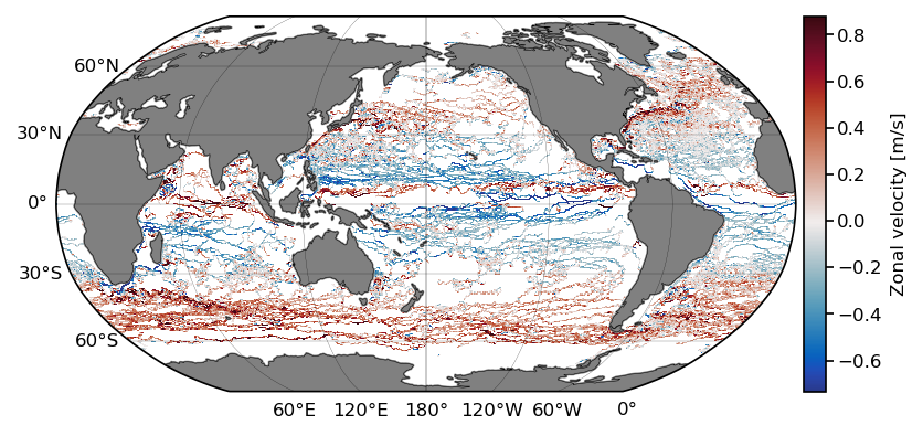
    summary:           Global Drifter Program hourly data

Xarray test 1: Geographical binning of any variable#

The first benchmark test implemented here is to compute statistics per geographical bins. Here we choose to compute the mean of the zonal velocity (ve) from all drifter estimates. From the previous cell, we can see that the size of the chunks were automatically set to the size of obs, leading to one chunk per variable. For this type of bin operation, one chunk is convenient because the complete zonal velocity ragged array variable will be loaded in memory in one operation. In order to perform operations per trajectory (shown below), we will instead set the size of the chunks to be the length of each trajectory, which here would have required subset_nb_drifters operation to load the same data.

Note: chunks should always align with the computation to optimize performance (more details in section 5.3.2).

In order to keep track of computing times of each test, we create a variable benchmark_times.

benchmark_times = np.zeros((3,3))  # 3 benchmark tests for the 3 different processing libraries

We calculate the mean zonal velocity using the binned_statistic_2d function from the stats module of the scipy package:

t0 = time.time()

lon = np.linspace(-180, 180, 360*2)
lat = np.linspace(-90, 90, 180*2)

ret = stats.binned_statistic_2d(ds.lon, 
                                ds.lat,
                                ds.ve,
                                statistic=np.nanmean, 
                                bins=[lon, lat])

benchmark_times[0,0] = time.time() - t0

We now plot the results:

x_c = np.convolve(lon, [0.5, 0.5], mode='valid')
y_c = np.convolve(lat, [0.5, 0.5], mode='valid')

# get 1st and 99th percentiles of values to plot to get a useful range for the colorscale
v1,v2 = np.nanpercentile(ret.statistic.T,[1,99])

fig = plt.figure(dpi=150)
ax = fig.add_subplot(1,1,1,projection=ccrs.Robinson(central_longitude=-180))
cmap = cmocean.tools.crop(cmocean.cm.balance, vmin=v1, vmax=v2, pivot=0)
pcm = ax.pcolormesh(x_c, y_c, 
                    ret.statistic.T, 
                    cmap=cmap, 
                    transform=ccrs.PlateCarree(),
                    vmin=v1, vmax=v2)

# gridlines and labels
gl = ax.gridlines(color='k', linewidth=0.1, linestyle='-',
                  xlocs=np.arange(-180, 181, 60), ylocs=np.arange(-90, 91, 30),
                  draw_labels=True)
gl.top_labels = False
gl.right_labels = False

# add land and coastline
ax.add_feature(cfeature.LAND, facecolor='grey', zorder=1)
ax.add_feature(cfeature.COASTLINE, linewidth=0.25, zorder=1)
divider = make_axes_locatable(ax)
cax = divider.append_axes("right", size="3%", pad=0.05, axes_class=plt.Axes)
cb = fig.colorbar(pcm, cax=cax);
cb.ax.set_ylabel('Zonal velocity [m/s]');

../../_images/PM_05_Accelerating_Lagrangian_analyses_of_oceanic_data_benchmarking_typical_workflows_37_0.png

Xarray test 2: Extract a given region#

Extracting a subregion of the dataset is also a very common operation. xarray provides efficient way to apply mask to the data. One important thing to note is that since we have two dimensions, a mask is applied on the obs as well as on the traj dimensions. We first define a function to do the data extraction:

def retrieve_region(ds, lon: list = None, lat: list = None, time: list = None) -> xr.Dataset:
    '''Subset the dataset for a region in space and time
    
    Args:
        ds: xarray Dataset
        lon: longitude slice of the subregion
        lat: latitude slice of the subregion
        time: tiem slice of the subregion
    
    Returns: 
        ds_subset: Dataset of the subregion
    '''
    
    # define the mask for the 'obs' dimension
    mask = np.ones(ds.dims['obs'], dtype='bool')

    if lon:
        mask &= (ds.coords['lon'] >= lon[0]).values
        mask &= (ds.coords['lon'] <= lon[1]).values

    if lat:
        mask &= (ds.coords['lat'] >= lat[0]).values
        mask &= (ds.coords['lat'] <= lat[1]).values

    if time:
        mask &= (ds.coords['time'] >= np.datetime64(time[0])).values
        mask &= (ds.coords['time'] <= np.datetime64(time[1])).values
    
    # define the mask for the 'traj' dimension using the ID numbers from the masked observation
    mask_id = np.in1d(ds.ID, np.unique(ds.ids[mask]))
    ds_subset = ds.isel(obs=np.where(mask)[0], traj=np.where(mask_id)[0])

    return ds_subset.compute()

Next we use this function to extract the data from the Gulf of Mexico for years 2000 to 2020:

t0 = time.time()

# we need to record the time for benchmarking in the end
lon = [-98, -78]
lat = [18, 31]
day0 = datetime(2000,1,1).strftime('%Y-%m-%d')
day1 = datetime(2020,12,31).strftime('%Y-%m-%d')
days = [day0, day1]
ds_subset = retrieve_region(ds, lon, lat, days)

benchmark_times[0,1] = time.time() - t0

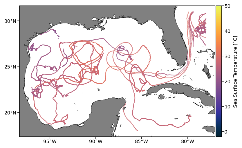
For visualization of the results, the sea surface temperature estimates along trajectories from the extracted subregion are plotted in the next cell.

fig = plt.figure(dpi=150)
ax = fig.add_subplot(1,1,1,projection=ccrs.PlateCarree())

# temperature data are in Kelvin so we convert to degree Celsius
pcm = ax.scatter(ds_subset.lon, ds_subset.lat, 
               s=0.05, c=ds_subset.sst-273.15, transform=ccrs.PlateCarree(),
               cmap=cmocean.cm.thermal, vmin=-2, vmax=50)

ax.add_feature(cfeature.LAND, facecolor='grey', zorder=1)
ax.add_feature(cfeature.COASTLINE, linewidth=0.25, zorder=1)
ax.set_xticks(np.arange(-95, -79, 5), crs=ccrs.PlateCarree())
ax.set_yticks([20, 25, 30], crs=ccrs.PlateCarree())
ax.xaxis.set_major_formatter(LongitudeFormatter())
ax.yaxis.set_major_formatter(LatitudeFormatter())
divider = make_axes_locatable(ax)
cax = divider.append_axes('right', size='3%', pad=0.02, axes_class=plt.Axes)
cb = fig.colorbar(pcm, cax=cax)
cb.set_label('Sea Surface Temperature [˚C]')

../../_images/PM_05_Accelerating_Lagrangian_analyses_of_oceanic_data_benchmarking_typical_workflows_43_0.png

Xarray test 3: Operations per trajectory#

Operations per trajectory#

As previously noted, to perform the same operation per trajectory, it is more efficient to align the chunks with the trajectories. This is done by settings the size of the chunks equal to the dimensions of the trajectories. However, here we need to know the lengths of all the trajectories in the order they are arranged in the ragged array before actually loading the dataset with xarray. This is clearly not practical as xarray does not provide an obvious mechanism to align the data chunks with specified indices.

rowsize = np.zeros(len(files), dtype='int')
for i, file in enumerate(files):
    with xr.open_dataset(file, decode_times=False) as ds_t:
        rowsize[i] = ds_t.sizes['obs']

ds.close()  # close previously loaded xr.Dataset

# align chunks of the dask array with the length of each individual trajectory
chunk_settings = {'obs': tuple(rowsize.tolist())}

ds = xr.open_dataset('data/gdp_subset.nc', chunks=chunk_settings)

Variables such as the longitude, are now split into subset_nb_drifters chunks which have different sizes and where the maximum size is indicated by the Shape characteristic of the xarray.DataArray objects. As an example for lon:

ds.lon

<xarray.DataArray 'lon' (obs: 4786301)>
dask.array<open_dataset-7f2a95543265e3b414ce19877f3d517clon, shape=(4786301,), dtype=float32, chunksize=(50655,), chunktype=numpy.ndarray>
Coordinates:
    lon      (obs) float32 dask.array<chunksize=(1095,), meta=np.ndarray>
    lat      (obs) float32 dask.array<chunksize=(1095,), meta=np.ndarray>
    time     (obs) datetime64[ns] dask.array<chunksize=(1095,), meta=np.ndarray>
    ids      (obs) int64 dask.array<chunksize=(1095,), meta=np.ndarray>
Dimensions without coordinates: obs
Attributes:
    long_name:  Longitude
    units:      degrees_east

Naturally, now loading a trajectory always require loading only one chunk.

i = 10
ds.lon.isel({'obs': slice(traj_idx[i], traj_idx[i+1])})

<xarray.DataArray 'lon' (obs: 4151)>
dask.array<getitem, shape=(4151,), dtype=float32, chunksize=(4151,), chunktype=numpy.ndarray>
Coordinates:
    lon      (obs) float32 dask.array<chunksize=(4151,), meta=np.ndarray>
    lat      (obs) float32 dask.array<chunksize=(4151,), meta=np.ndarray>
    time     (obs) datetime64[ns] dask.array<chunksize=(4151,), meta=np.ndarray>
    ids      (obs) int64 dask.array<chunksize=(4151,), meta=np.ndarray>
Dimensions without coordinates: obs
Attributes:
    long_name:  Longitude
    units:      degrees_east

Simple operation by chunks (or blocks)#

To perform arbitrary operation per trajectory, we can now use map_blocks() that applies a function per chunk (block is also used for chunks). In the example below we simply define the function func that calculates the mean of each block of an array x. Note that this requires loading nb_subset_drifters chunks and applying the operation.

def func(x):
    return np.array([np.nanmean(x)])

stats_traj = ds.sst.data.map_blocks(func).compute() # apply to sst variable

/var/folders/jh/92r7zqw159xbv25hk5fbrzgw0000gp/T/ipykernel_2540/1074368307.py:2: RuntimeWarning: Mean of empty slice
  return np.array([np.nanmean(x)])

stats_traj[:10]

array([275.79956, 280.2327 , 277.82953, 282.86588, 293.74094, 293.33972,
       287.9495 , 271.2664 , 293.4779 , 300.82187], dtype=float32)

More complex operation where dimensions can change between input and output#

Alternatively, one can use the xarray function apply_ufunc to map a function per chunks. In this case, the function to be applied can be a bit more complex, but this method gives more flexibility to handle the input and output formats and dimensions of the function.

In a first example, the eastward velocity is passed as an argument by chunk to the function which will calculate the anomaly per trajectory. The length of the output will be of the same length as the input. Please note here that:

The input and output sizes are not modified.
An argument must be passed to the function. It shouldn’t be ds.ve (the xarray DataArray), but the ds.ve.data (the underlying dask core data array) must be used.

def per_chunk_anomaly(array):
    # MUST return an array (https://github.com/dask/dask/issues/8822)
    return array.map_blocks(lambda x: x-np.nanmean(x), chunks=array.chunks)

# here the apply_ufunc functions takes the function just defined above(per_chunk_anomaly)
# and the data to which apply that function
ret = xr.apply_ufunc(
    per_chunk_anomaly,
    ds.ve.data,  # .data to retrieve the underlying chunked dask array
    input_core_dims=[['obs']],
    output_core_dims=[['obs']],
    dask='allowed'
).compute()

And display some results:

display(ret)  # only a few values will be shown by default
display(len(ret))  # length of the output should be same as length of input

array([0.02569735, 0.02569735, 0.02599735, ..., 0.13741829, 0.13441828,
       0.12031829], dtype=float32)

In a second example, we calculates mean() values per trajectory. This means that for our datasets consisting of nb_subset_drifters chunks, ttput will have nb_subset_drifters values, that is one value per chunk. In other words, the length of the output will be different from the length of the input.

def per_chunk_mean(array):
    nchunks = len(array.chunks[0])
    output_chunks = ([1] * nchunks,) # 1 value per chunk
    return array.map_blocks(lambda x: np.nanmean(x, keepdims=True), chunks=output_chunks)

ret = xr.apply_ufunc(
    per_chunk_mean,
    ds.ve.data,
    input_core_dims=[['obs']],  # input dimension to the per_block function
    output_core_dims=[['obs']], # output still has one dimension
    exclude_dims=set(['obs']),  # size of x changes so it has to be in the exclude_dims param
    dask='allowed',
).compute()

And display some results:

display(ret[:10])  # show only first 10 values
display(len(ret))  # length of output should be the number of trajectories

array([-0.03099735,  0.14964446,  0.152546  ,  0.15595299,  0.01793322,
       -0.01830383,  0.03096705, -0.03741267, -0.00138449,  0.03001278],
      dtype=float32)

In a last example, we estimate ocean velocity rotary spectra of the complex-valued time series u+vi via the periodogram method (and using the NumPy fft function). Here, the combination of the two methods apply_ufunc and map_blocks is a powerful tool which can serve as templates for a range of advanced processing applied per trajectory.

First, we create the new complex-valued variable cv which inherits the chunks from ve and vn:

ds = ds.assign(cv = ds['ve'] + 1j*ds['vn'])
ds.cv

<xarray.DataArray 'cv' (obs: 4786301)>
dask.array<add, shape=(4786301,), dtype=complex64, chunksize=(50655,), chunktype=numpy.ndarray>
Coordinates:
    lon      (obs) float32 dask.array<chunksize=(1095,), meta=np.ndarray>
    lat      (obs) float32 dask.array<chunksize=(1095,), meta=np.ndarray>
    time     (obs) datetime64[ns] dask.array<chunksize=(1095,), meta=np.ndarray>
    ids      (obs) int64 dask.array<chunksize=(1095,), meta=np.ndarray>
Dimensions without coordinates: obs

def per_chunk_periodogram(array):
    dt = 1/24  # [-]
    return array.map_blocks(lambda x: dt*np.abs(np.fft.fft(x))**2, chunks=array.chunks)

Here we benchmark this last, more complex, operation:

t0 = time.time()

ret = xr.apply_ufunc(
    per_chunk_periodogram,
    ds['cv'].data,
    input_core_dims=[["obs"]],  # input dimension to the per_block function
    output_core_dims=[["obs"]],  # output still has one dimension
    dask='allowed'
).compute()

benchmark_times[0,2] = time.time() - t0

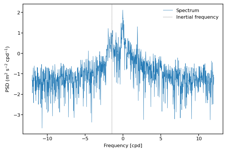
The return variable is the same length as ds['cv'], and is a ragged array of estimated rotary spectra by the periodogram method.

(Please note: the periodogram is not a good spectral estimator at all and alternative methods such as multitaper methods should be used to estimate spectra. Please also note that we assumed that the individual trajectories were gap-free at regular hourly intervals which is required to apply a FFT. However, some velocity time series have gaps, in which case the FFT calculation is not valid)

Display one example spectrum:

i = 0   # drifter index

# calculate inertial frequency in cycle per day [cpd] from the mean latitude of trajectory
omega = 7.2921159e-5  # Earth's rotation rate [rad/s]
seconds_per_day = 60*60*24  # [s]
fi = -2*omega*(seconds_per_day/(2*np.pi))*np.sin(np.radians(ds.lat[traj_idx[i]:traj_idx[i+1]]).mean().compute())

# define frequency scale/abscissa
dt = 1/24  # [-]
f = np.fft.fftfreq(int(ds.rowsize[i].compute()), dt) 
ss = np.log10(ret[traj_idx[i]:traj_idx[i+1]])  # spectrum of the ith trajectory 

fig = plt.figure(dpi=150)
ax = fig.add_subplot(1,1,1)

h1, = ax.plot(np.fft.fftshift(f), np.fft.fftshift(ss), scaley=True, label='Spectrum', linewidth=0.5)
h2 = ax.axvline(x=fi,color='k',linestyle=':', label='Inertial frequency', linewidth=0.5)
ax.legend(frameon=False)
ax.set_ylabel('PSD (m$^2$ s$^{-2}$ cpd$^{-1}$)')
ax.set_xlabel('Frequency [cpd]');

../../_images/PM_05_Accelerating_Lagrangian_analyses_of_oceanic_data_benchmarking_typical_workflows_82_0.png

At this stage it is necessary to clear the memory (RAM) of the Python process because in the next step, the data are fully loaded in memory by using Pandas.

del ds, ds_subset, ret, traj_idx, stats_traj, rowsize, x_c, y_c

Pandas#

In this section, we test the use of the Pandas package for our Lagrangian data. Since the previously-created NetCDF file containing the ragged array has two dimensions ['traj'] and ['obs'], it cannot be read directly into the table structure of a pandas.DataFrame(). As a workaround, we load the data with xarray, drop the ['traj'] dimension, and convert the resulting data to a pandas.DataFrame(). The disadvantage is that it requires to form a second dataset with the dimension['traj'] to have access to all variables (not presented here).

df = xr.open_dataset('data/gdp_subset.nc').drop_dims('traj').to_pandas()  # only contains the variables with dimension ['obs']

In this case, the data is organized in a table format where each variable is associated with a column, and each row contains one observation. A DataFrame is easy to quickly look at, with the .head(), .tail() functions as an example:

df.head()

	ve	vn	gap	err_lat	err_lon	err_ve	err_vn	drogue_status	sst	sst1	...	err_sst	err_sst1	err_sst2	flg_sst	flg_sst1	flg_sst2	lon	lat	time	ids
obs
0	-0.0053	0.0004	15638.0	0.00391	0.00797	0.0650	0.0279	False	273.471985	274.126007	...	0.074	0.224	0.236	5	5	4	-52.393002	47.307461	2001-05-01 08:00:00	2592
1	-0.0053	0.0007	15638.0	0.00345	0.00676	0.0603	0.0284	False	273.100006	273.760010	...	0.077	0.158	0.185	5	5	4	-52.393070	47.307590	2001-05-01 09:00:00	2592
2	-0.0050	0.0015	15638.0	0.00313	0.00586	0.0548	0.0290	False	272.869995	273.513000	...	0.086	0.113	0.142	5	5	4	-52.392960	47.307861	2001-05-01 10:00:00	2592
3	-0.0037	0.0035	15638.0	0.00288	0.00503	0.0511	0.0297	False	272.752991	273.334015	...	0.096	0.089	0.123	5	5	4	-52.392208	47.308449	2001-05-01 11:00:00	2592
4	-0.0044	0.0031	13651.0	0.00292	0.00475	0.0509	0.0313	False	272.743988	273.213013	...	0.102	0.078	0.118	5	5	4	-52.391151	47.309021	2001-05-01 12:00:00	2592

5 rows × 21 columns

print(f'This subset contains {len(np.unique(df.ids))} drifters and {len(df):,} observations.')

This subset contains 500 drifters and 4,786,301 observations.

Pandas test 1: Geographical binning of any variable#

Here we reconduct the first bench test: calculate the mean zonal velocity from all drifters of the dataset.

t0 = time.time()

lon = np.linspace(-180, 180, 360*2)
lat = np.linspace(-90, 90, 180*2)

ret = stats.binned_statistic_2d(df.lon, 
                                df.lat, 
                                df.ve,
                                statistic=np.nanmean, # can pass any function()
                                bins=[lon, lat])

benchmark_times[1,0] = time.time() - t0

x_c = np.convolve(lon, [0.5, 0.5], mode='valid')
y_c = np.convolve(lat, [0.5, 0.5], mode='valid')

# get 1st and 99th percentiles of values to plot to get a useful range for the colorscale
v1,v2 = np.nanpercentile(ret.statistic.T,[1,99])

fig = plt.figure(dpi=150)
ax = fig.add_subplot(1,1,1,projection=ccrs.Robinson(central_longitude=-180))
cmap = cmocean.tools.crop(cmocean.cm.balance, vmin=v1, vmax=v2, pivot=0)
pcm = ax.pcolormesh(x_c, y_c, 
                    ret.statistic.T, 
                    cmap=cmap, 
                    transform=ccrs.PlateCarree(),
                    vmin=v1, vmax=v2)

# gridlines and labels
gl = ax.gridlines(color='k', linewidth=0.1, linestyle='-',
                  xlocs=np.arange(-180, 181, 60), ylocs=np.arange(-90, 91, 30),
                  draw_labels=True)
gl.top_labels = False
gl.right_labels = False
# add land and coastline
ax.add_feature(cfeature.LAND, facecolor='grey', zorder=1)
ax.add_feature(cfeature.COASTLINE, linewidth=0.25, zorder=1)
divider = make_axes_locatable(ax)
cax = divider.append_axes("right", size="3%", pad=0.05, axes_class=plt.Axes)
cb = fig.colorbar(pcm, cax=cax);
cb.ax.set_ylabel('Zonal velocity [m/s]');

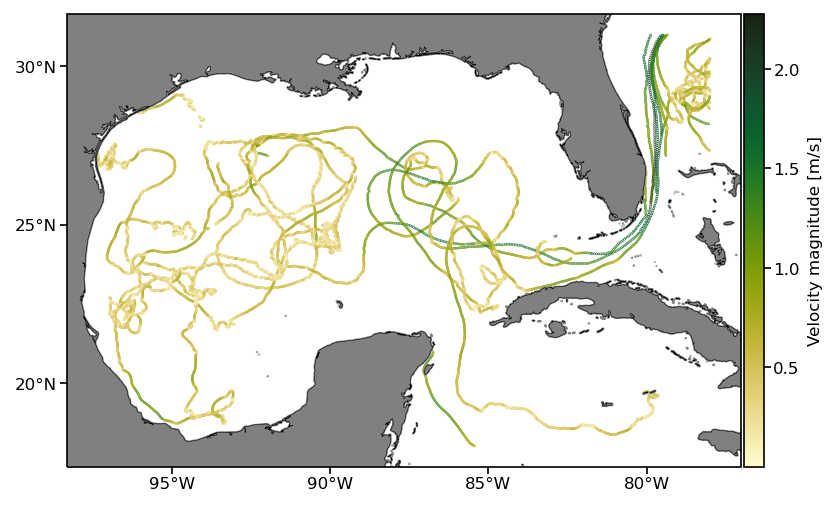
../../_images/PM_05_Accelerating_Lagrangian_analyses_of_oceanic_data_benchmarking_typical_workflows_92_0.png

Pandas test 2: Extract a given region#

The extraction of a region is slightly simpler with Pandas than with xarray, because the same mask can be applied to all variables of interest that share the obs dimension.

def retrieve_region_pd(df, lon: list = None, lat: list = None, time: list = None):
    '''Subset the dataset for a region in space and time
    
    Args:
        df: Pandas DataFrame
        lon: longitude slice of the subregion
        lat: latitude slice of the subregion
        time: tiem slice of the subregion
    
    Returns: 
        ds_subset: Dataset of the subregion
    '''
    mask = functools.reduce(np.logical_and, 
                            (
                                df.lon >= lon[0], 
                                df.lon <= lon[1],
                                df.lat >= lat[0],
                                df.lat <= lat[1],
                                df.time >= day0,
                                df.time <= day1,
                            )
                           )
    
    return df.loc[mask]

t0 = time.time()

lon = [-98, -78]
lat = [18, 31]
day0 = datetime(2000,1,1)
day1 = datetime(2020,12,31)
days = [day0, day1]
df_subset = retrieve_region_pd(df, lon, lat, days)

benchmark_times[1,1] = time.time() - t0

df_subset.head()

	ve	vn	gap	err_lat	err_lon	err_ve	err_vn	drogue_status	sst	sst1	...	err_sst	err_sst1	err_sst2	flg_sst	flg_sst1	flg_sst2	lon	lat	time	ids
obs
902352	-0.3192	-0.0632	10886.0	0.00611	0.01212	0.1262	0.0633	False	301.339996	301.382996	...	0.022	0.007	0.019	5	5	5	-78.007187	30.198179	2006-09-15 14:00:00	54388
902353	-0.4248	-0.0653	10886.0	0.00193	0.01652	0.1244	0.0656	False	301.377014	301.386993	...	0.021	0.007	0.018	5	5	2	-78.036041	30.196760	2006-09-15 15:00:00	54388
902354	-0.1182	-0.0115	4925.0	0.00219	0.01249	0.1813	0.0548	False	301.417999	301.390015	...	0.018	0.006	0.016	5	5	5	-78.044693	30.193790	2006-09-15 16:00:00	54388
902355	-0.0863	-0.0425	1210.0	0.00063	0.00932	0.1501	0.0463	False	301.457001	301.391998	...	0.015	0.006	0.014	5	5	5	-78.048553	30.192690	2006-09-15 17:00:00	54388
902356	0.0080	-0.0562	4925.0	0.00415	0.00690	0.1936	0.0922	False	301.487000	301.394012	...	0.013	0.005	0.012	5	5	5	-78.045929	30.191130	2006-09-15 18:00:00	54388

5 rows × 21 columns

Here we plot the result as before but displaying the speed for each data point:

fig = plt.figure(dpi=150)
ax = fig.add_subplot(1,1,1,projection=ccrs.PlateCarree())

pcm = ax.scatter(df_subset.lon, df_subset.lat, 
               s=0.05, c=np.sqrt(df_subset.ve**2+df_subset.vn**2), transform=ccrs.PlateCarree(),
               cmap=cmocean.cm.speed)

ax.add_feature(cfeature.LAND, facecolor='grey', zorder=1)
ax.add_feature(cfeature.COASTLINE, linewidth=0.25, zorder=1)
ax.set_xticks(np.arange(-95, -79, 5), crs=ccrs.PlateCarree())
ax.set_yticks([20, 25, 30], crs=ccrs.PlateCarree())
ax.xaxis.set_major_formatter(LongitudeFormatter())
ax.yaxis.set_major_formatter(LatitudeFormatter())
divider = make_axes_locatable(ax)
cax = divider.append_axes('right', size='3%', pad=0.02, axes_class=plt.Axes)
cb = fig.colorbar(pcm, cax=cax)
cb.set_label('Velocity magnitude [m/s]')

../../_images/PM_05_Accelerating_Lagrangian_analyses_of_oceanic_data_benchmarking_typical_workflows_98_0.png

Pandas test 3: Single statistic per trajectory#

Single operation per trajectory can be easily implemented in a Pandas DataFrame by locating the drifter ID by index (iloc) or by value (loc).

i = 10  # drifter index

df.iloc[np.where(df['ids'] == np.unique(df['ids'])[i])].mean(numeric_only=False)

ve                                    0.143713
vn                                   -0.042606
gap                                14790.94043
err_lat                               0.007155
err_lon                                0.01117
err_ve                                0.095038
err_vn                                0.064061
drogue_status                         0.998073
sst                                 285.678101
sst1                                285.681427
sst2                                 -0.003311
err_sst                               0.070594
err_sst1                              0.024895
err_sst2                              0.063991
flg_sst                               4.997591
flg_sst1                              4.997591
flg_sst2                              3.857866
lon                                 -45.807869
lat                                 -45.521275
time             2003-03-17 05:04:36.656227328
ids                                    27131.0
dtype: object

Assuming we know a drifter ID id_ex (here we simply use the value associated to the i^th index above), we can retrieve the associated data by value as follow.

id_ex = np.unique(df['ids'])[i]
id_ex

df.loc[df['ids'] == id_ex].mean(numeric_only=False)

ve                                    0.143713
vn                                   -0.042606
gap                                14790.94043
err_lat                               0.007155
err_lon                                0.01117
err_ve                                0.095038
err_vn                                0.064061
drogue_status                         0.998073
sst                                 285.678101
sst1                                285.681427
sst2                                 -0.003311
err_sst                               0.070594
err_sst1                              0.024895
err_sst2                              0.063991
flg_sst                               4.997591
flg_sst1                              4.997591
flg_sst2                              3.857866
lon                                 -45.807869
lat                                 -45.521275
time             2003-03-17 05:04:36.656227328
ids                                    27131.0
dtype: object

For more complicated operations per trajectory, the pandas groupby() function allows us to split the DataFrame. Applied to the ids['obs'] (which repeat the ID of a drifter for each of its observations), we can obtain a grouped object containing one trajectory per group. Following this operation, one can apply a predefined set of operations, such as mean(), or any user defined functions using .apply(). As before, we provide an example where we can calculate the mean of SST per trajectory, and another example of estimating velocity spectra by the periodogram method.

ret = df.groupby("ids").sst.mean()
ret

ids
2592        275.799561
6428        280.232697
13566       277.829529
17927       282.865875
18706       293.740936
               ...    
68243870    273.882111
68244460    273.744598
68244730    273.515564
68246720    296.040009
68248530    286.112793
Name: sst, Length: 500, dtype: float32

Again, to estimate the velocity spectra we have to create the new complex-valued variable cv from ve and vn:

df['cv'] = df['ve'] + 1j*df['vn']

And calculate the periodogram per trajectory using this new variable:

def periodogram_per_group(array):
    dt = 1/24
    return dt*np.abs(np.fft.fft(array))**2

t0 = time.time()

ret = df.groupby("ids").cv.apply(periodogram_per_group)

benchmark_times[1,2] = time.time() - t0

This time, the results are stored into a dictionary where the keys are the drifters’ ID:

ret

ids
2592        [48.01623216121766, 52.74661085729767, 4.63967...
6428        [341830.5755422627, 53330.50826245666, 857.134...
13566       [46152.48004791965, 6588.974982702436, 1458.62...
17927       [325605.62376754, 63676.24022864982, 11794.261...
18706       [1076.965552542786, 773.9372866187755, 311.397...
                                  ...                        
68243870    [127.7695912061453, 215.20477509848652, 315.08...
68244460    [301.4939495649164, 64.02978051130118, 424.069...
68244730    [383.1069530335443, 67.31997165755263, 7.50842...
68246720    [308.7263083474708, 1125.3042873617292, 4771.3...
68248530    [49.898529559024354, 2.2134116883119983, 15.66...
Name: cv, Length: 500, dtype: object

As an example, we display the first 10 values of the sprctrum for drifter id_ex:

ret[id_ex][:10]

array([16131.45017614, 16040.80300053,  3017.6902432 ,  6700.41755415,
         311.93297982,  1555.5981903 ,   757.26867001,  7200.28268359,
         891.88959794,  1036.35997949])

del df, df_subset, ret, x_c, y_c  # again free the memory before the next section

Awkward Array#

Awkward Array is a library for nested, variable-sized data, including arbitrary-length lists, records, mixed types, and missing data, using NumPy-like idioms. Such arrays are dynamically typed (defined at runtime as a function of the variable to store), but operations on them are compiled into machine code and therefore executes faster than regular interpreted Python function. This allow to generalizes NumPy array manipulation routines, even with variable-sized data.

A schematic view of the data structure is presented in the figure below. The higher level ak.Array and ak.Record hides the nested structure of the data structure, but can always be accessed with ak.Array.layout (or ds_ak.layout in our case). This structure also stores parameters or metadata such as units, long name, etc. associated with the data. The library stores data into standard NumPyArray alongside a ListOffsetArray for fast and efficient access to variables, even with nonuniform data length.

The main advantages of Awkward Array are:

the indexing is already taken care of by the library, e.g. sst[400] returns the sea surface temperature along the 401^st trajectory;
ability to efficiently perform operations per trajectory;
easy integration with Numba (demonstrated below in section 7.4).

An Awkward array can easily be created by reading our NetCDF file:

ds_ak = create_ak(xr.open_dataset('data/gdp_subset.nc', decode_times=False))

Awkward Arrays supports N-dimensional datasets by storing nested arrays. The main dataset contains variables (type = subset_nb_drifters * {various type}) containing the metadata.

ds_ak

<Array [{ID: 2592, rowsize: 1095, ... ] type='500 * struct[["ID", "rowsize", "lo...'>

Awkward Array doesn’t (yet!) have an html representation of its structure, but it is possible to list the fields.

ds_ak.fields  # list of fields/variables

['ID',
 'rowsize',
 'location_type',
 'WMO',
 'expno',
 'deploy_date',
 'deploy_lat',
 'deploy_lon',
 'end_date',
 'end_lat',
 'end_lon',
 'drogue_lost_date',
 'type_death',
 'type_buoy',
 'DeploymentShip',
 'DeploymentStatus',
 'BuoyTypeManufacturer',
 'BuoyTypeSensorArray',
 'CurrentProgram',
 'PurchaserFunding',
 'SensorUpgrade',
 'Transmissions',
 'DeployingCountry',
 'DeploymentComments',
 'ManufactureYear',
 'ManufactureMonth',
 'ManufactureSensorType',
 'ManufactureVoltage',
 'FloatDiameter',
 'SubsfcFloatPresence',
 'DrogueType',
 'DrogueLength',
 'DrogueBallast',
 'DragAreaAboveDrogue',
 'DragAreaOfDrogue',
 'DragAreaRatio',
 'DrogueCenterDepth',
 'DrogueDetectSensor',
 'obs']

If we peak inside one of the field (or variable), we can see the associated type. For example, the drifters’ ID have a type=subset_nb_drifters * int64.

ds_ak.ID  # one variable

<Array [2592, 6428, ... 68246720, 68248530] type='500 * int64[parameters={"attrs...'>

If we display the last field ‘obs’, we can see that it is a nested Awkward Array and contains all variables with type=(subset_nb_drifters * var * dtype) containing data along trajectories.

ds_ak.obs

<Array [{lon: [-52.4, -52.4, -52.4, ... 5, 5]}] type='500 * {"lon": [var * float...'>

The library includes the function ak.flatten(), similar to np.flatten() to concatenate all observations for one variable into a unidimensional array. As an example, with ‘sst’:

print(f'Total length of the data inside \'obs\' field \'sst\' are {len(ak.flatten(ds_ak.obs.sst)):,}.')
ak.flatten(ds_ak.obs.sst)

Total length of the data inside 'obs' field 'sst' are 4,786,301.

<Array [273, 273, 273, 273, ... 287, 288, 288] type='4786301 * float32'>

A nested structure is utilized to efficiently store N-dimensional dataset, in our case we first have the fields with dimension ['traj'], followed by the fields with dimension ['obs'] stored inside the array ds_ak.obs.

ds_ak.obs.fields

['lon',
 'lat',
 'time',
 'ids',
 've',
 'vn',
 'gap',
 'err_lat',
 'err_lon',
 'err_ve',
 'err_vn',
 'drogue_status',
 'sst',
 'sst1',
 'sst2',
 'err_sst',
 'err_sst1',
 'err_sst2',
 'flg_sst',
 'flg_sst1',
 'flg_sst2']

For example, the type of the sst field, stored at ds_ak.obs.sst, is 17324 * var * float32. This means that there are 17324 trajectories of variable size of float32`.

ds_ak.obs.sst

<Array [[273, 273, 273, ... 287, 288, 288]] type='500 * [var * float32, paramete...'>

The data along the trajectory of a specific drifter can easily be retrieved using an index.

i = 0
ds_ak.obs.sst[i]

<Array [273, 273, 273, 273, ... 280, 280, nan] type='1095 * float32'>

The same data can be extracted from the drifter ID:

id_ex = ds_ak.ID[i] # id of the ith trajectory as an example
display(id_ex)
i = np.where(ds_ak.ID == id_ex)[0][0]
ds_ak.obs.sst[i]

<Array [273, 273, 273, 273, ... 280, 280, nan] type='1095 * float32'>

And the data along a specific trajectory can be accessed using a second index. As an example, the first sst value of the i^th trajectory:

ds_ak.obs.sst[i][0]  # [K]

273.47198486328125

Metadata or attributes are store for the global Array ds_ak.layout.parameters, as well as for each individual variable (ds_ak.obs.sst.layout.parameters), similarly to global attributes and variable attributes in a NetCDF file. Those attributes are stored as a parameter in the ak.RecordArray (obtained with the .layout member), which summarizes the data fields, the types, and the shapes of the data itself.

ds_ak.layout.parameters

{'attrs': {'title': 'Global Drifter Program hourly drifting buoy collection',
  'history': 'Version 2.00.  Metadata from dirall.dat and deplog.dat',
  'Conventions': 'CF-1.6',
  'date_created': '2022-05-20T14:48:40.763710',
  'publisher_name': 'GDP Drifter DAC',
  'publisher_email': 'aoml.dftr@noaa.gov',
  'publisher_url': 'https://www.aoml.noaa.gov/phod/gdp',
  'licence': 'MIT License',
  'processing_level': 'Level 2 QC by GDP drifter DAC',
  'metadata_link': 'https://www.aoml.noaa.gov/phod/dac/dirall.html',
  'contributor_name': 'NOAA Global Drifter Program',
  'contributor_role': 'Data Acquisition Center',
  'institution': 'NOAA Atlantic Oceanographic and Meteorological Laboratory',
  'acknowledgement': 'Elipot et al. (2022) to be submitted. Elipot et al. (2016). Global Drifter Program quality-controlled hourly interpolated data from ocean surface drifting buoys, version 2.00. NOAA National Centers for Environmental Information. https://agupubs.onlinelibrary.wiley.com/doi/full/10.1002/2016JC011716TBA. Accessed [date].',
  'summary': 'Global Drifter Program hourly data'}}

ds_ak.obs.sst.layout.parameters

{'attrs': {'long_name': 'Fitted sea water temperature',
  'units': 'Kelvin',
  'comments': 'Estimated near-surface sea water temperature from drifting buoy measurements. It is the sum of the fitted near-surface non-diurnal sea water temperature and fitted diurnal sea water temperature anomaly. Discrepancies may occur because of rounding.'}}

Awkward Array test 1: Geographical binning of any variable#

Again, we reconduct the first bench test: calculate the mean zonal velocity from all drifters of the dataset. For operations apply on the full dataset, we use the ak.flatten() function to retrieve the underlying unidimensional NumPy array containing all the observations for all drifters.

t0 = time.time()

lon = np.linspace(-180, 180, 360 * 2)
lat = np.linspace(-90, 90, 180 * 2)

ret = stats.binned_statistic_2d(ak.flatten(ds_ak.obs.lon, axis=1), 
                                ak.flatten(ds_ak.obs.lat, axis=1), 
                                ak.flatten(ds_ak.obs.ve, axis=1),
                                statistic=np.nanmean,
                                bins=[lon, lat])
        
benchmark_times[2,0] = time.time() - t0

x_c = np.convolve(lon, [0.5, 0.5], mode='valid')
y_c = np.convolve(lat, [0.5, 0.5], mode='valid')

# get 1st and 99th percentiles of values to plot to get a useful range for the colorscale
v1,v2 = np.nanpercentile(ret.statistic.T,[1,99])

fig = plt.figure(dpi=150)
ax = fig.add_subplot(1,1,1,projection=ccrs.Robinson(central_longitude=-180))
cmap = cmocean.tools.crop(cmocean.cm.balance, vmin=v1, vmax=v2, pivot=0)
pcm = ax.pcolormesh(x_c, y_c, 
                    ret.statistic.T, 
                    cmap=cmap, 
                    transform=ccrs.PlateCarree(),
                    vmin=v1, vmax=v2)

# gridlines and labels
gl = ax.gridlines(color='k', linewidth=0.1, linestyle='-',
                  xlocs=np.arange(-180, 181, 60), ylocs=np.arange(-90, 91, 30),
                  draw_labels=True)
gl.top_labels = False
gl.right_labels = False
# add land and coastline
ax.add_feature(cfeature.LAND, facecolor='grey', zorder=1)
ax.add_feature(cfeature.COASTLINE, linewidth=0.25, zorder=1)
divider = make_axes_locatable(ax)
cax = divider.append_axes("right", size="3%", pad=0.05, axes_class=plt.Axes)
cb = fig.colorbar(pcm, cax=cax);
cb.ax.set_ylabel('Zonal velocity [m/s]');

../../_images/PM_05_Accelerating_Lagrangian_analyses_of_oceanic_data_benchmarking_typical_workflows_145_0.png

Awkward Array test 2: Extract a given region#

With Awkward Array, the extraction of a subregion is slightly more complex than with Pandas, since here the dataset contains both variables with dimension ['traj'] and variables with dimension ['obs']. Note that comparisons can be performed on the bidimensional non-regular ak.Array (e.g. ds.obs.lon, ds.obs.lat, ds.obs.time) without looping.

def retrieve_region_ak(ds: ak.Array, lon: list = None, lat: list = None, days: list = None) -> ak.Array:
    '''Subset the dataset for a region in space and time
    
    Args:
        ds: Awkward Array
        lon: longitude slice of the subregion
        lat: latitude slice of the subregion
        days: days slice of the subregion
    
    Returns: 
        ds_subset: Dataset of the subregion
    '''
    mask = functools.reduce(np.logical_and, 
                            (
                                ds.obs.lon >= lon[0], 
                                ds.obs.lon <= lon[1],
                                ds.obs.lat >= lat[0],
                                ds.obs.lat <= lat[1],
                                ds.obs.time >= days[0],
                                ds.obs.time <= days[1],
                            )
                           )
    
    ds_s = ak.copy(ds)
    mask_id = np.in1d(ds_s.ID, np.unique(ak.flatten(ds_s.obs.ids[mask])))
    ds_s = ds_s[mask_id]  # mask for variables with dimension ['traj']
    ds_s.obs = ds_s.obs[mask[mask_id]] # mask for variables with dimension ['obs']
    
    return ds_s

t0 = time.time()

lon = [-98, -78]
lat = [18, 31]
day0 = (datetime(2000,1,1) - datetime(1970,1,1)).total_seconds()
day1 = (datetime(2020,12,31) - datetime(1970,1,1)).total_seconds()
days = [day0, day1]
ds_subset = retrieve_region_ak(ds_ak, lon, lat, days)

benchmark_times[2,1] = time.time() - t0

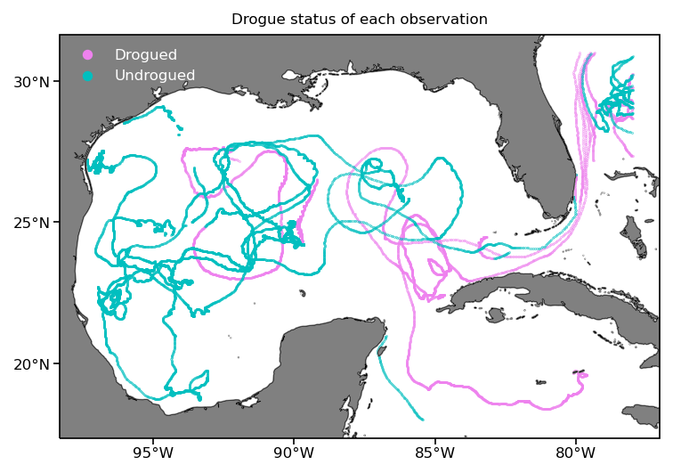
Here we plot the result as before but displaying the drogue status of drifters along their trajectory. Note: the drogue is a sea anchor centered at 15 m depth that can become detached, after which the drifter is more strongly affected by surface winds and waves.

fig = plt.figure(dpi=150)
ax = fig.add_subplot(1,1,1,projection=ccrs.PlateCarree())

cond = ds_subset.obs.drogue_status  # True: drogued, False: undrogued
pcm = ax.scatter(ak.flatten(ds_subset.obs.lon[cond]), ak.flatten(ds_subset.obs.lat[cond]), 
               s=0.05, c='violet', transform=ccrs.PlateCarree(), label='Drogued')

pcm = ax.scatter(ak.flatten(ds_subset.obs.lon[~cond]), ak.flatten(ds_subset.obs.lat[~cond]), 
               s=0.05, c='c', transform=ccrs.PlateCarree(), label='Undrogued')

ax.add_feature(cfeature.LAND, facecolor='grey', zorder=1)
ax.add_feature(cfeature.COASTLINE, linewidth=0.25, zorder=1)
ax.set_xticks(np.arange(-95, -79, 5), crs=ccrs.PlateCarree())
ax.set_yticks([20, 25, 30], crs=ccrs.PlateCarree())
ax.xaxis.set_major_formatter(LongitudeFormatter())
ax.yaxis.set_major_formatter(LatitudeFormatter())
ax.set_title('Drogue status of each observation', size=8);
ax.legend(markerscale=20, labelcolor='w', frameon=False);

../../_images/PM_05_Accelerating_Lagrangian_analyses_of_oceanic_data_benchmarking_typical_workflows_150_0.png

Awkward Array test 3: Single statistic per trajectory#

Without the need for indices, we can perform reduction operation per trajectory directly with Awkward array, which simplify considerably the notations, and should ease the development of new functionality.

Note: At this point, the dataset ds_ak is loaded in memory, which explains the speed of the operations. For larger dataset that cannot be held completely in memory, an option could be to interface with Dask, currently under development.

avg_sst = np.zeros(len(ds_ak.obs))
for i, s in enumerate(ds_ak.obs.sst):
    avg_sst[i] = np.nanmean(s)
avg_sst[:10]

/Users/pmiron/miniforge3/envs/research/lib/python3.9/site-packages/awkward/_connect/_numpy.py:36: RuntimeWarning: Mean of empty slice
  out = func(*args, **kwargs)

array([275.79956055, 280.23269653, 277.82952881, 282.86587524,
       293.74093628, 293.33972168, 287.94949341, 271.26638794,
       293.47790527, 300.8218689 ])

For basic operations, we can also use Awkward Array to perform averages along a specific axis. In our situation, ak.mean(lon, axis=1) perform the same mean operation per trajectory, see that the type is then reduced to subset_nb_drifters * float64.

*Note: The nan versions of those operations (ak.nanmean, ak.nanstd, ak.nanmax, etc.) is not yet available but is currently in development.

avg_lon = ak.mean(ds_ak.obs.lon, axis=1)
avg_lon

<Array [-53.5, -6.68, -74.5, ... -151, -143] type='500 * ?float64'>

Applying more complex operation can be easily implemented with simple for-loop, since the indexing is taken care by Awkward Array.

def periodogram_per_traj(uv):
    dt = 1/24
    d = []    
    for i in range(0, len(uv)):
        d.append(dt*np.abs(np.fft.fft(uv[i]))**2)
    return d

t0 = time.time()

ret = periodogram_per_traj(
    ds_ak.obs.ve + 1j*ds_ak.obs.vn
)

benchmark_times[2,2] = time.time() - t0

Each element of the list ret now contains the fast Fourier transform of the complex velocity u + iv per trajectory:

ret[:5]

[<Array [48, 52.7, 4.64, ... 16, 58.1, 131] type='1095 * float64'>,
 <Array [3.42e+05, 5.33e+04, ... 3.41e+03] type='19132 * float64'>,
 <Array [4.62e+04, 6.59e+03, ... 3.11e+03] type='6631 * float64'>,
 <Array [3.26e+05, 6.37e+04, ... 5.03e+04] type='17906 * float64'>,
 <Array [1.08e+03, 774, 311, ... 540, 2.21e+03] type='5738 * float64'>]

Numba#

Awkward Array can be combined with Numba to accelerate calculations. Here, the goal is not to show the most efficient way of performing a calculation, but to present how simply adding the numba decorator @nb.njit to a function can improved the performance by order of magnitude(s).

Here we show an example that calculates the kinetic energy of a drifter trajectory from its velocity time series:

def kinetic_energy(u, v):
    ke = np.zeros(len(u))
    for i in range(0, len(u)):
        ke[i] = np.sqrt(u[i]**2 + v[i]**2)
    return ke
        
@nb.njit
def kinetic_energy_nb(u, v):
    ke = np.zeros(len(u))
    for i in range(0, len(u)):
        ke[i] = np.sqrt(u[i]**2 + v[i]**2)
    return ke

# select a random trajectory
i = 10

%%time
ke = kinetic_energy(ds_ak.obs.ve[i], ds_ak.obs.vn[i])

CPU times: user 160 ms, sys: 2.02 ms, total: 162 ms
Wall time: 164 ms

The function is compiled just in time when we execute the function for the first time, future executions are numba fast.

kinetic_energy_nb(ds_ak.obs.ve[i], ds_ak.obs.vn[i])

array([0.18460563, 0.19851099, 0.19387937, ..., 0.32900888, 0.32915556,
       0.32936901])

%%timeit -r10 -n10
ke2 = kinetic_energy_nb(ds_ak.obs.ve[i], ds_ak.obs.vn[i])

705 µs ± 78.2 µs per loop (mean ± std. dev. of 10 runs, 10 loops each)

This results in more than a 500x sped up (!) for the same function simply by adding the @nb.njit decorators!

del ds_ak, ret, x_c, y_c

Discussion#

We presented a commonly used Lagrangian oceanographic dataset (the GDP dataset) which is currently available as individual NetCDF files (one of the means of distribution). Next, we presented an efficient data structure, the contiguous ragged array, to combine the variables from these individual NetCDF files. We then compared three different packages–xarray , Pandas, and Awkward Array—by performing typical Lagrangian workflow tasks.

Xarray

xarray is a well-known and established package used to perform operations on N-Dimensional datasets. It is natively integrated with Dask for parallel computing(not demonstrated in this Notebook), and allows users to lazy load data when the dataset is larger than the available memory of the computing environment.

However, it is not typically used with contiguous ragged array, so applying operation per trajectory requires to manually index through the dataset. One possibility is to set the size of the Dask chunks equals to the size of the trajectories, which allows for mapping operation in parallel per trajectory. However, the typical high number of chunks is less than ideal: it hinders performance since a simple operation like computing mean values across a dataset containing n trajectories requires to conduct n reading operation on the data file.

Pandas

Pandas is a predominantly used Python data analysis package. Since it is designed to perform operations on tabular data, it is required to form two DataFrame tables to represent the complete GDP dataset: one containing the variables with one value per trajectory (['traj']), and a second one containing the variables with one value per observations along the trajectory (['obs']). Unfortunately, this creates a separation the data and their metadata.

In this Notebook we used only a subset of the GDP dataset by randomly selecting only 500 trajectories. The data were therefore entirely contained within the active memory and the operations performed were fast and written in an elegant and intuitive fashion. However, if these operations are conducted on the entire dataset (17324 trajectories) we found the execution to be much slower than with xarray or Awkward Array which seem able to manage memory much more efficiently.

Awkward Array

Awkward Array is a novel library specifically designed to deal with ragged and heterogeneous data (in type or size). With the example of the heterogeneous GDP dataset, we find that this library simplifies considerably Lagrangian analysis. Furthermore, integration with Numba allows to speed up calculations without major redesign. We anticipate that these two advantages will lead to faster development of Lagrangian analysis functions as part of the CloudDrift project.

Initially developed for particle physics applications, Awkward Array is missing some useful features (e.g. html representation, import from NetCDF, and especially Dask integration) when compared to more mature libraries like xarray or Pandas. During the development of this Notebook, we had the opportunity to engage with the authors of this library, and we plan on collaborating to fill those gaps during the development the clouddrift libraries. We believe that this collaboration will elevate both projects, which are sponsored by the National Science Foundation during similar time frame (Awkward Array #2103945).

Benchmark speed#

The following figure presents the benchmark times obtain for the current execution. As a comparison, we include a reference time (black dashed line) obtained on a 2021 Mac Mini with a 8 cores Apple M1 ARM processor, 16GB of RAM, running macOS Monterey 12.3.

Note: user should expect slower time on a Binder or Google Colab environment. We understand that a lot of factors can influence the results of this benchmark, and it might not be the most accurate when running on a Cloud environment, or on a local cluster with multiple users. We still believe it gives an interesting view of the performance of the three selected libraries.

ref_times = np.array([[3.26, 0.46, 0.23],  # [s]
                      [3.21, 0.06, 0.38],
                      [3.22, 0.13, 0.32]])

fig = plt.figure(dpi=150)
ax = fig.add_subplot(1,1,1)

index = np.arange(0,3)
bar_width = 0.2

t1 = plt.bar(index, benchmark_times[0,:], bar_width,
                 color='violet',
                 label='Xarray')

t2 = plt.bar(index + bar_width, benchmark_times[1,:], bar_width,
                 color='limegreen',
                 label='Pandas')

t3 = plt.bar(index + 2*bar_width, benchmark_times[2,:], bar_width,
                 color='aqua',
                 label='Awkward Array')

# add reference times
for i in range(0, len(index)):
    x = np.array([index[i], index[i] + bar_width, index[i] + 2*bar_width])
    ax.plot(x, ref_times[:,i], 'k', linewidth=0.75, linestyle='dashed', label='Reference time (Apple M1, 16GB)')

plt.xlabel('Workflow tests')
plt.ylabel('Elapsed time [s] (lower is better)')
plt.title('Benchmark times per library')
plt.xticks(index + bar_width, ('Binning', 'Region extraction', 'Periodogram per trajectory'))
handles, labels = plt.gca().get_legend_handles_labels()
by_label = dict(zip(labels, handles))
plt.legend(by_label.values(), by_label.keys(), frameon=False)

<matplotlib.legend.Legend at 0x17ff4c8e0>

../../_images/PM_05_Accelerating_Lagrangian_analyses_of_oceanic_data_benchmarking_typical_workflows_176_1.png

Feedback#

If you ran this notebook on a local computer, please help us guide the development of CloudDrift by sharing one or all following points to the discussion thread on Github Discussion:

your comments on the ease of use of Xarray and/or Pandas and/or Awkward Arrays for Lagrangian data analysis;
the figure of your benchmark timings in the previous cell;
your system information generated by executing the next cell;
any other comments!

Thanks!

# summary of the system for log purpose
# inspired from https://stackoverflow.com/a/58420504/1558320
def getSystemInfo():
    info={}
    info['platform']=platform.system()
    info['platform-release']=platform.release()
    info['platform-version']=platform.version()
    info['architecture']=platform.machine()
    info['processor']=platform.processor()
    try:
        info['frequency']=psutil.cpu_freq(percpu=False)
    except:
        info['frequency']='N/A'
    info['cores']=psutil.cpu_count(logical=False)
    info['threads']=psutil.cpu_count(logical=True)
    info['ram']=str(round(psutil.virtual_memory().total / (1024.0 **3)))+" GB"
    return info

getSystemInfo()

{'platform': 'Darwin',
 'platform-release': '21.4.0',
 'platform-version': 'Darwin Kernel Version 21.4.0: Fri Mar 18 00:47:26 PDT 2022; root:xnu-8020.101.4~15/RELEASE_ARM64_T8101',
 'architecture': 'arm64',
 'processor': 'arm',
 'frequency': 'N/A',
 'cores': 8,
 'threads': 8,
 'ram': '16 GB'}

Future development#

We hope you will follow the development of CloudDrift, and encourage everyone to share this Notebook as well as submit feedback and comments to team members.

References#

Elipot et al. (2016), “A global surface drifter dataset at hourly resolution”, J. Geophys. Res. Oceans, 121, doi:10.1002/2016JC011716
Hansen, D. V., & Poulain, P. M. (1996). Quality control and interpolations of WOCE-TOGA drifter data. Journal of Atmospheric and Oceanic Technology, 13(4), 900-909, doi:10.1175/1520-0426(1996)013%3C0900:QCAIOW%3E2.0.CO;2

EarthCube 2022 Call for Notebooks

Accelerating Lagrangian analyses of oceanic data: benchmarking typical workflows

Contents