Intro to Argovis’ API
Contents
Intro to Argovis’ API#
Purpose#
The Argovis project (argovis.colorado.edu, [1]) is upgrading its API, with a new design that better supports expressive, targeted search across multiple data sources, including Argo floats [2, 3], GO-SHIP profiles [4], and more. This new API is intended to enable co-location studies across datasets and efficiently scoped download of exactly the data researchers need. The purpose of this notebook is to illustrate some of the key features of this API as it is being developed; please note that this API is still under development and will evolve further before full release (including access to other datasets), and that helper functions here are examples only and will be superseded by a python library in future. Please send comments, feedback and feature requests to the team at argovis@colorado.edu.
Technical contributions#
API development to access point data in a new schema (e.g. oceanic profiles)
Alpha demo of the new Earth system data API, including:
Co-location and cross referencing of disparate data sources
Querying and downloading data or metadata subsets for exactly the measurements of interest (e.g. oxygen profiles in the ocean), within the metadata space (lat / lon / time, data source, etc) of interest.
Methodology#
A new hierarchical JSON schema for describing generic Earth-system point data was developed in collaboration between Argo and GO-SHIP data experts, into which e.g. Argo and GO-SHIP data were cast and indexed in Mongodb. This allows for convenient and powerful cross-indexing of these data for performing the co-location searches of interest.
On top of this data structure, a new RESTful API was developed that leverages the OpenAPI standard for specification and documentation of point data search routes. Emphasis was placed on creating the ability to make targeted queries that return only the data of interest, filtered by user-specified metadata and data search parameters, in order to leverage server-side resources on behalf of users and allow them to download only the data of interest to them, thus enabling rapid, interactive analysis building.
In the following, we will demo some of the data queries that are possible with the new API.
Results#
Ocean profile data is queried, returned and plotted, filtered by data source, geography, and available measurements.
Argo core and BGC measurements are co-located with GO-SHIP WOCE lines of interest.
Co-located measurements are plotted and compared.
Examples of filtering measurement data by QC flag, and interpolating measurements onto regular depth profiles are presented.
Funding#
Argovis is currently funded by two NSF awards:
Award1 = {“agency”: “US National Science Foundation”, “award_code”: “1928305”, “award_URL”: ” https://www.nsf.gov/awardsearch/showAward?AWD_ID=1928305&HistoricalAwards=false “}
Award2 = {“agency”: “US National Science Foundation”, “award_code”: “2026776”, “award_URL”: ” http://www.nsf.gov/awardsearch/showAward?AWD_ID=2026776&HistoricalAwards=false “}
Keywords#
keywords= [“Argovis”,“Argo”,”floats”,”GO-SHIP”,“oceanic profiles”,’hydrographic data”,”profiling floats”,”in-situ observations”]
Citation#
Mills, W., Giglio, D., Scanderbeg, M., Tucker, T. (2022). Intro to Argovis’ API. A DOI will be assigned after review.
Suggested next steps#
Python library of helper functions and wrappers: this notebook leverages some simple helper functions for wrapping API calls; these should be formalized and expanded as a fully unit tested and versioned python library distributed on Pypi.
Schema finalization: the current database implements a release candidate of our point data schema; this will likely be updated based on early feedback.
Data source expansion: the current database includes a selection of Argo and GO-SHIP data, but has been designed to be highly extensible; integrating more data sources (e.g. tropical cyclone, atmospheric river, satellite, and gridded data) will be pursued as ongoing work.
Acknowledgements#
GO-SHIP data were included in Argovis as part of a collaboration with Sarah Purkey, Steve Diggs, Lynne Merchant, Karen Stocks, and Andrew Barna (NSF award #2026776).
This iteration of Argovis is hosted at the University of Colorado, Boudler, on the CU Platform Engineering team’s OpenShift Kubernetes platform. The authors thank and acknowledge the whole platform team at CU for their consistent support.
Setup#
Library import#
We begin by importing some typical libraries, as well as some examples of custom helper functions that wrap the Argovis API:
#data processing
import numpy as np
import pandas as pd
from datetime import datetime, timedelta
import time

#data visualization
%matplotlib inline
import matplotlib.pylab as plt
%matplotlib inline

import warnings
warnings.filterwarnings('ignore')
Local library import#
##### import local functions
# for data processing
from utilities_NSF_EC2022 import create_url, get_data_from_url, get_info_from_df,get_data_for_timeRange, \
                                    polygon_lon_lat, mask_QC, simple_plot, qc, interpolate
# for data visualization
from utilities_NSF_EC2022 import set_ax_label, \
                                 set_map_and_plot_locations_withColor
Parameter definitions#
Next, let’s populate some useful parameters for our API. We’ll store the root of our API in URL_PREFIX, and pass our API key around in API_KEY. If you don’t have an Argovis API key, you can get one for free at https://argovis-keygen.colorado.edu/ API keys allow us to allocate our resources fairly to all our users. API_KEY can be also left empty '' (as in the cell below), yet in this case the user may exceed API request limits (and get HTTP 403 errors), depending on system load at the time.
# prefix to use with all API queries
URL_PREFIX = 'https://argovis-api.colorado.edu'
API_KEY   = ''
Let’s also declare some space-time variables we’ll use to filter our search results by in the following examples. Dates are encoded as ISO 8601 UTC datestrings, and polygons are defined as lists of [lon, lat] pairs; to construct a polygon interactively:
visit argovis.colorado.edu
draw a shape
click on the purple shaded area of the region of interest (not on a dot)
from the pop up window, go “to Selection page”
from the url of the selection shape, copy the shape, i.e. [copy_all_this_inside_outer_brackets] after ‘shape=’
startDate = '2021-04-20T00:00:00Z'
endDate   = '2021-05-02T00:00:00Z'
# To see what this polygon looks like, visit https://argovis.colorado.edu/ng/home?mapProj=WM&presRange=%5B0,2000%5D&selectionStartDate=2022-03-31T22:30:45Z&selectionEndDate=2022-04-14T22:30:45Z&threeDayEndDate=2022-04-12T22:30:45&shapes=%5B%5B%5B22.105999,-76.289063%5D,%5B26.902477,-72.597656%5D,%5B26.084682,-66.395555%5D,%5B25.005973,-60.292969%5D,%5B10.833306,-65.566406%5D,%5B11.942098,-72.133142%5D,%5B22.105999,-76.289063%5D%5D%5D&includeRealtime=true&onlyBGC=false&onlyDeep=false&threeDayToggle=false
polygon = '[[-76.289063,22.105999],[-72.597656,26.902477],[-66.395555,26.084682],[-60.292969,25.005973],[-65.566406,10.833306],[-72.133142,11.942098],[-76.289063,22.105999]]'

# helper function parameters
## list of parameters to extract from dataframes to dictionaries for plotting, see get_info_from_df
info_to_store = ['lon','lat','date','cols_bySource','ids','woce_line']

## repackaging of polygon coordinates for plotting, see set_map_and_plot_locations_withColor
polygon_lon_lat_dict = polygon_lon_lat(polygon_str=polygon)
Data import#
Note that due to the nature of this notebook as an API technical demo, data import is performed throughout the following examples. Helper functions are provided to wrap API calls, but expert users are encouraged to access the API directly, as informed by the API documentation here.
Data processing and analysis#
Co-location examples#
One of Argovis’ goals is to enable co-location studies: quickly seeing when and where two or more datasets intersect, possibly providing crosschecks or other mutually supporting data. In what follows, we’ll see some examples of co-locating Argo and GO-SHIP measurements in the polygon we defined above.
Data source searching & negation search#
First, let’s try selecting a few different sources of data, like Argo core [3], Argo BGC [3], and GO-SHIP [4] measurements, and plotting their co-location. See the helper functions for detailed implementation of the API wrapper, but here we’re leveraging the API’s /profiles endpoint and its time range (via startDate= and endDate=), data source (via source=) and region (via polygon=) metadata filtering.
source_all = ['argo_core','argo_bgc','cchdo_go-ship']
for isource in source_all:
    bfr_df = get_data_for_timeRange(startDate=startDate,endDate=endDate, \
                                url_prefix=URL_PREFIX+'/profiles?', \
                                myAPIkey=API_KEY, \
                                source=isource, \
                                polygon=polygon, \
                                dt_tag='365d',writeFlag=True)
    if not bfr_df.empty:
        bfr_info = get_info_from_df(df=bfr_df,info_to_store=info_to_store)
        ###### let's plot the polygon and the profile locations color coded by source
        set_map_and_plot_locations_withColor(lon=bfr_info['lon'],lat=bfr_info['lat'], \
                                     cols=bfr_info['cols_bySource'], \
                                     polygon_lon_lat_dict=polygon_lon_lat_dict)
        plt.title('source: ' + isource,fontsize=28)
Number of items: 50
https://argovis-api.colorado.edu/profiles?&startDate=2021-04-20T00:00:00Z&endDate=2021-05-02T23:59:59Z&polygon=[[-76.289063,22.105999],[-72.597656,26.902477],[-66.395555,26.084682],[-60.292969,25.005973],[-65.566406,10.833306],[-72.133142,11.942098],[-76.289063,22.105999]]&source=argo_core
Number of items: 4
https://argovis-api.colorado.edu/profiles?&startDate=2021-04-20T00:00:00Z&endDate=2021-05-02T23:59:59Z&polygon=[[-76.289063,22.105999],[-72.597656,26.902477],[-66.395555,26.084682],[-60.292969,25.005973],[-65.566406,10.833306],[-72.133142,11.942098],[-76.289063,22.105999]]&source=argo_bgc
Number of items: 46
https://argovis-api.colorado.edu/profiles?&startDate=2021-04-20T00:00:00Z&endDate=2021-05-02T23:59:59Z&polygon=[[-76.289063,22.105999],[-72.597656,26.902477],[-66.395555,26.084682],[-60.292969,25.005973],[-65.566406,10.833306],[-72.133142,11.942098],[-76.289063,22.105999]]&source=cchdo_go-ship

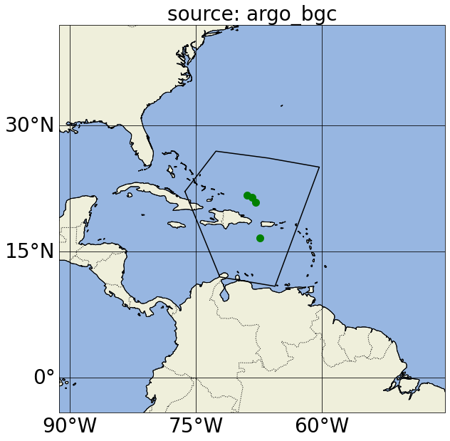
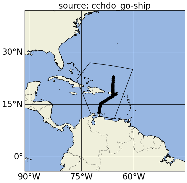
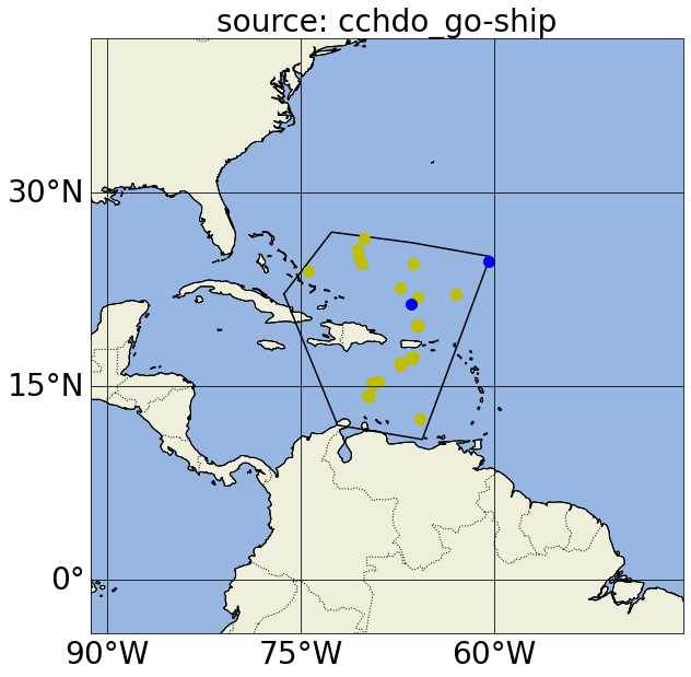
In these plots, yellow points correspond to Argo profiles without BGC variables or measurements deeper than 2500 dbar; green points correspond to Argo BGC profiles; blue points correspond to Deep Argo profiles (with measurements deeper than 2500 dbar); and black dots correspond to GO-SHIP profiles.
Notice in the first map, we actually got argo_bgc, argo_deep and argo_core profiles when we asked for argo_core; this is because Argo floats that measure BGC variables and/or sample below 2000m will also carry the argo_core tag. If we want to exclude profiles that include argo_bgc variables, we can use Argovis’ negation search in the source filter (please refer to the previous paragraph for the color of the dots in the next cell):
bfr_df = get_data_for_timeRange(startDate=startDate,endDate=endDate, \
                            url_prefix=URL_PREFIX+'/profiles?', \
                            myAPIkey=API_KEY, \
                            source='argo_core,~argo_bgc', \
                            polygon=polygon, \
                            dt_tag='365d',writeFlag=True)
if not bfr_df.empty:
    bfr_info = get_info_from_df(df=bfr_df,info_to_store=info_to_store)
    ###### let's plot the polygon and the profile locations color coded by source
    set_map_and_plot_locations_withColor(lon=bfr_info['lon'],lat=bfr_info['lat'], \
                                 cols=bfr_info['cols_bySource'], \
                                 polygon_lon_lat_dict=polygon_lon_lat_dict)
    plt.title('source: ' + isource,fontsize=28)
Number of items: 46
https://argovis-api.colorado.edu/profiles?&startDate=2021-04-20T00:00:00Z&endDate=2021-05-02T23:59:59Z&polygon=[[-76.289063,22.105999],[-72.597656,26.902477],[-66.395555,26.084682],[-60.292969,25.005973],[-65.566406,10.833306],[-72.133142,11.942098],[-76.289063,22.105999]]&source=argo_core,~argo_bgc
Now (map above) we don’t have profiles that include argo_bgc variables, as desired. If we want an account of the different types of Argo profiles in a region, we can iterate through these source parameters:
'argo_core,~argo_bgc,~argo_deep''argo_bgc,~argo_deep''argo_deep,~argo_bgc''argo_bgc,argo_deep'
Counting the profiles for each query, we would know how many profiles only have core variables (exclusive of deep and BGC variables), how many profiles have BGC variables exclusive of deep measurements, how many profiles have deep measurements exclusive of BGC variables, and how many profiles have both BGC variables and deep measurements, respectively. We note that argo_deep profiles are tagged as any profile with levels deeper than 2500 dbar, and therefore will also carry an argo_core and (if applicable) argo_bgc source tag. If we want to check for edge cases when a BGC profile file is available yet a core file is not, we can use the parameter 'argo_bgc,~argo_core' (this should not happen).
Searching by available data#
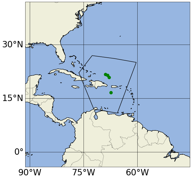
We often only want profiles that have data of interest. Argovis features the ability to perform exactly this type of search, providing metadata and data only for profiles with the measurements we need. Let’s look for profiles in our region of interest that have dissolved oxygen and pressure measurements, by using the data filter. Also note adding metadata-only to the filter list tells Argovis to look for profiles that have the data listed, but only actually return the corresponding metadata for those profiles:
df = get_data_for_timeRange(startDate=startDate,endDate=endDate, \
                                url_prefix=URL_PREFIX+'/profiles?', \
                                myAPIkey=API_KEY, \
                                data='doxy,pres,metadata-only', \
                                polygon=polygon, \
                                dt_tag='100d',writeFlag=True)
if not df.empty:
    if 'df_all' in locals():
        df_all = pd.concat([df_all,df],ignore_index=True)
    else:
        df_all = df

# store some info
info_d_reg = get_info_from_df(df=df_all,info_to_store=info_to_store)

# delete df_all
del df_all

###### let's plot the polygon and profile locations color coded by source
set_map_and_plot_locations_withColor(lon=info_d_reg['lon'],lat=info_d_reg['lat'], \
                                     cols=info_d_reg['cols_bySource'], \
                                     polygon_lon_lat_dict=polygon_lon_lat_dict)
Number of items: 4
https://argovis-api.colorado.edu/profiles?&startDate=2021-04-20T00:00:00Z&endDate=2021-05-02T23:59:59Z&polygon=[[-76.289063,22.105999],[-72.597656,26.902477],[-66.395555,26.084682],[-60.292969,25.005973],[-65.566406,10.833306],[-72.133142,11.942098],[-76.289063,22.105999]]&data=doxy,pres,metadata-only
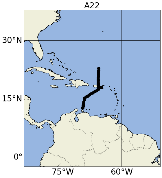
We can perform a similar search, this time demanding data be only from a particular WOCE (World Ocean Circulation Experiment) line with the woceline= filter (instead of querying profiles in a region as done previously):
if 'df_d1' in locals():
    del df_d1

df = get_data_for_timeRange(startDate=startDate,endDate=endDate, \
                                url_prefix=URL_PREFIX+'/profiles?', \
                                myAPIkey=API_KEY, \
                                data='pres,doxy_ctd,metadata-only', \
                                woceline='A22', \
                                dt_tag='365d',writeFlag=True)
if not df.empty:
    if 'df_d1' in locals():
        df_d1 = pd.concat([df_d1,df],ignore_index=True)
    else:
        df_d1 = df
# store some info
info_d1 = get_info_from_df(df=df_d1,info_to_store=info_to_store)

font = {'weight' : 'normal',
        'size'   : 24}

plt.rc('font', **font)
set_map_and_plot_locations_withColor(lon=info_d1['lon'],lat=info_d1['lat'], \
                                     cols=info_d1['cols_bySource'], \
                                     polygon_lon_lat_dict=[])
plt.title('A22',fontsize=28)
Number of items: 46
https://argovis-api.colorado.edu/profiles?&startDate=2021-04-20T00:00:00Z&endDate=2021-05-02T23:59:59Z&data=pres,doxy_ctd,metadata-only&woceline=A22
Text(0.5, 1.0, 'A22')
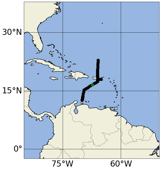
Proximity search#
Now that we’ve identified some information from this WOCE line of interest, we can use Argovis’ proximity search to find nearby Argo profiles, via the radius and center pair of query parameters, which together search for profiles within a given distance of a centerpoint. Here we also use the metadata-only flag to data, so we get profiles that contain pres and doxy, but for now only actually download their metadata:
delta_days = 3.5

if 'df_d2' in locals():
    del df_d2

lst_id_pairs_d1 = []
lst_id_pairs_d2 = []

for i in np.arange(0,len(info_d1['lon'])):
    time.sleep(.2)
    d = get_data_for_timeRange(startDate=(datetime.strptime(info_d1['date'][i],'%Y-%m-%dT%H:%M:%SZ')- \
                                          timedelta(days=delta_days)).strftime('%Y-%m-%dT%H:%M:%SZ'),
                               endDate=(datetime.strptime(info_d1['date'][i],'%Y-%m-%dT%H:%M:%SZ')+ \
                                          timedelta(days=delta_days)).strftime('%Y-%m-%dT%H:%M:%SZ'), \
                               myAPIkey=API_KEY, \
                               center=str(info_d1['lon'][i])+','+str(info_d1['lat'][i]), \
                               radius_km='50', \
                               url_prefix=URL_PREFIX+'/profiles?', \
                               data='pres,doxy,metadata-only', \
                               source='argo_core', \
                               dt_tag='365d',writeFlag=False)
    if not d.empty:
        #info_d2 = {**info_d2, **get_info_from_df(df=d,info_to_store=info_to_store)}
        #list_d2 = list_d2 + [d]
        if 'df_d2' in locals():
            df_d2 = pd.concat([df_d2,d],ignore_index=True)
        else:
            df_d2 = d
        lst_id_pairs_d2.append(d['_id'].tolist())
        lst_id_pairs_d1.append(info_d1['ids'][i])

info_d2=get_info_from_df(df=df_d2,info_to_store=info_to_store)

###### let's plot the profile locations color coded by source
set_map_and_plot_locations_withColor(lon=info_d1['lon']+info_d2['lon'],lat=info_d1['lat']+info_d2['lat'], \
                                     cols=info_d1['cols_bySource']+info_d2['cols_bySource'])
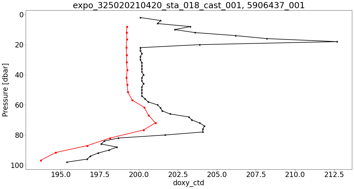
Finally, now that we’ve found Argo and GO-SHIP profiles that both measure dissolved oxygen, we can download the measurements of interest, plot the two and compare:
font = {'weight' : 'normal',
        'size'   : 24}

plt.rc('font', **font)

col_d1 = 'k'
col_d2 = 'r'

var_d = ['doxy_ctd', 'doxy']

mrk_sz1 = 7
mrk_sz2 = 5

mrk_type1 = '*'
mrk_type2 = 's'

presRange ='0,100'

for i in np.arange(0,len(lst_id_pairs_d1),1):
    ids_bfr1 = lst_id_pairs_d1[i]
    ids_bfr2 = lst_id_pairs_d2[i]
    if isinstance(ids_bfr1,str):
        ids_bfr1 = [ids_bfr1]
    if isinstance(ids_bfr2,str):
        ids_bfr2 = [ids_bfr2]

    fig = plt.figure(figsize=(20,10))
    fig_close = True

    if 'bfr_title' in locals():
        del bfr_title

    # plot
    for isource in [1,2]:
        if 'ids_bfr' in locals():
            del ids_bfr
        ids_bfr = eval('ids_bfr'+str(isource))
        for j in ids_bfr:
            bfr = pd.DataFrame(get_data_from_url(url=URL_PREFIX+'/profiles?&data='+var_d[isource-1]+',pres&id='+j+'&presRange='+presRange,\
                                                 myAPIkey=API_KEY,writeFlag=False))
            if 'bfr_df' in locals():
                del bfr_df

            for j_df in bfr['data']:
                if not 'bfr_df' in locals():
                    bfr_df = pd.DataFrame(j_df)
                else:
                    bfr_df = pd.concat([bfr_df,j_df],ignore_index=True)
            if var_d[isource-1] in bfr_df.keys():
                bfr_df2plt = bfr_df[bfr_df.eval(var_d[isource-1]).notnull()]
                plt.plot(bfr_df2plt[var_d[isource-1]],bfr_df2plt['pres'], \
                         marker=eval('mrk_type'+str(isource)),markersize=eval('mrk_sz'+str(isource)),color=eval('col_d'+str(isource)),linewidth=2)
                if isource ==2:
                    fig_close = False
                if not 'bfr_title' in locals():
                    bfr_title = j
                else:
                    bfr_title = bfr_title + ', ' + j
    plt.gca().invert_yaxis()
    plt.title(bfr_title)
    plt.xlabel(set_ax_label(var_d[0]))
    plt.ylabel(set_ax_label('pres'))
    if fig_close:
        plt.close(fig)
QC filtering#
Argovis offers QC flags for data whenever available as elements in a profile’s data array, but by default does not make any filtering decisions based on those flags. This example will show you how to filter your data by corresponding QC.
See ref. table 2 in section 4.1 of http://www.argodatamgt.org/content/download/15699/102401/file/argo-quality-control-manual-version2.8.pdf for a description of Argo QC flag interpretations.
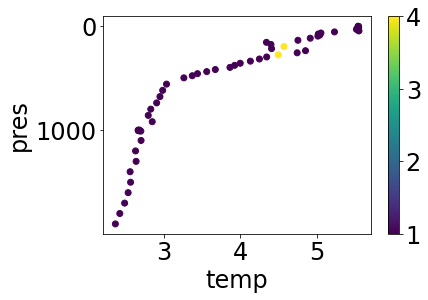
First, let’s get some data that has a couple of bad temperature measurements. Be sure to also ask for the QC variable temp_argoqc in your data query:
url = create_url(URL_PREFIX+'/profiles?', profile_id='3900321_108', data='pres,temp,temp_argoqc')
profile = get_data_from_url(url,API_KEY)[0]
Lets’s see what this temperature profile looks like in a simple plot that colors points by QC level:
simple_plot(profile, 'temp', 'temp_argoqc')
As noted, there are a couple of levels with QC > 1, which we might not want. Let’s filter those off so we can be completely confident in the data we’re using with another simple masking function, and then plot the result:
mp = mask_QC(profile, 'temp', [1])
simple_plot(mp, 'temp', 'temp_argoqc')
Levels with QC > 1 have been suppressed, leaving us with only top-quality data. For the curious, have a look at the definition of mask_QC; an important design pattern illustrated there is that the function both takes and returns a dictionary that matches the JSON schema specification of an Argovis profile object; therefore, this function can be safely combined with other functions with a similar signature in a profile processing pipeline.
mask_QC provides fine-grained control of QC filtering one variable at a time, but we can also use the convenience function qc to quickly scrub all the data in a profile. As a prerequisite, we must request QC data to go with every data variable; Argo QC data [5] for variable x is always found in x_argoqc, while CCHDO QC [6] is marked x_woceqc.
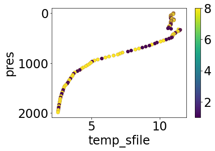
url = create_url(URL_PREFIX+'/profiles?', profile_id='2902115_144', data='pres,pres_argoqc,chla,chla_argoqc,temp_sfile,temp_sfile_argoqc')
profile = get_data_from_url(url,API_KEY)[0]
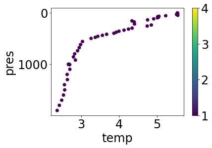
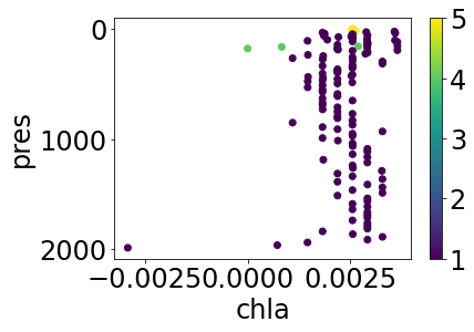
Let’s have a look at the BGC temperature and chlorophyll as they appear without QC filtering:
simple_plot(profile, 'temp_sfile', 'temp_sfile_argoqc')

simple_plot(profile, 'chla', 'chla_argoqc')
Apply the default cleaning (i.e. for argo profiles, we exclude measurements with QC > 1) to quickly tidy up, and replot:
cleaned = qc(profile)
simple_plot(cleaned, 'temp_sfile', 'temp_sfile_argoqc')
simple_plot(cleaned, 'chla', 'chla_argoqc')
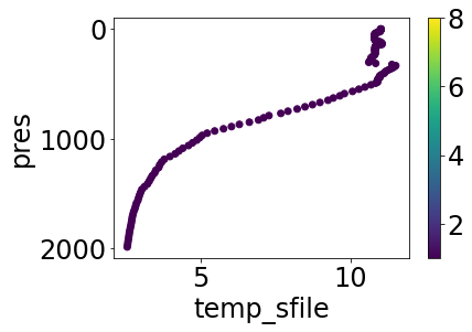
This worked quickly and easily, but if we look again at the original plots of this profile, most of the flagged levels for BGC temperature are QC=8, which indicates estimated, and not necessarily bad, data (for more information on Argo QC flags, see [5]). We can provide our cleaning function with custom levels to keep more points if desired:
partially_cleaned = qc(profile,[('temp_sfile',[1,8])])
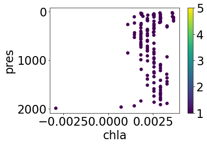
simple_plot(partially_cleaned, 'temp_sfile', 'temp_sfile_argoqc')
simple_plot(partially_cleaned, 'chla', 'chla_argoqc')

We get the estimated temperature measurements, but none of the high-flag chlorophyll.
Interpolation of profiles measurements to pressure levels of interest#
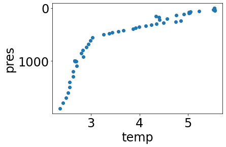
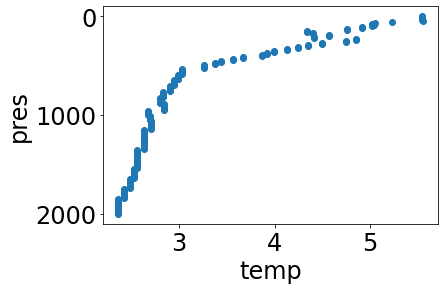
At times we may wish to interpolate data to a set of standard pressure levels, rather than keep whatever pressure levels a profile presents. The convenience function interpolate performs this for us. Let’s begin by fetching a profile as usual, and remember what its temperature plot looks like:
url = create_url(URL_PREFIX+'/profiles?', profile_id='3900321_108', data='pres,temp,temp_argoqc')
profile = get_data_from_url(url,API_KEY)[0]
simple_plot(profile, 'temp')
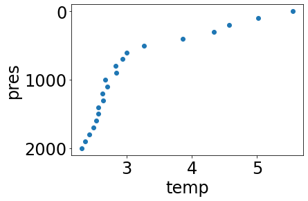
Use the interpolate function to interpolate every data variable in the profile to a set number of levels, every 100 dbar from 0 to 2000 dbar (e.g. approximately in the top 2000m):
interpolated_profile = interpolate(profile, list(range(0,2001))[0::100])
simple_plot(interpolated_profile, 'temp')
Note a few facts about interpolated profiles:
All QC information is dropped, as there is no meaningful way to interpolate QC flags. Therefore, it’s best to do any QC cleaning you desire before interpolation.
profile.data_warnings will include the flag
data_interpolatedto indicate a profile’s data has been interpolated in this fashion.By default, pchip intepolation is performed.
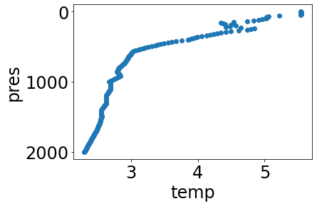
In addition to pchip, linear interpolation and nearest-neighbor are also available:
linear_interpolated_profile = interpolate(profile, list(range(0,2001))[0::10], method='linear')
simple_plot(linear_interpolated_profile, 'temp')
nn_interpolated_profile = interpolate(profile, list(range(0,2001))[0::10], method='nearest')
simple_plot(nn_interpolated_profile, 'temp')
References#
Tucker, T., Giglio, D., Scanderbeg, M., & Shen, S. S. P. (2020). Argovis: A Web Application for Fast Delivery, Visualization, and Analysis of Argo Data, Journal of Atmospheric and Oceanic Technology, 37(3), 401-416. doi:10.1175/JTECH-D-19-0041.1.
Argo (2000). Argo float data and metadata from Global Data Assembly Centre (Argo GDAC). SEANOE. doi:10.17882/42182.
https://cchdo.github.io/hdo-assets/documentation/manuals/pdf/90_1/chap4.pdf