GSEP Event Catalog and Time Series Dataset
Contents
GSEP Event Catalog and Time Series Dataset#
Purpose#
Solar Energetic Particle (SEP) events are radiation storms of particle fluxes comprising electrons, protons, and heavier ions from the Sun. SEP events are known to originate in large eruptions such as solar flares (SFs) and coronal mass ejections (CMEs). SEP events are essential to understand and forecast because (i) SEPs determine the dosage exposure on astronauts and spacecraft equipment outside the Earth’s magnetosphere; (ii) There is a sudden enhancement in space around Earth’s radiation environment during an SEP event; (iii) Solar protons with energies >100 Mega electronvolts (MeV) can penetrate the Earth’s upper atmosphere.
Multiple space and ground-based missions currently obtain in-situ solar particle composition and energy spectra fluxes. The time intensities of particle fluxes are used to define and characterize SEP events based on enhancements above a nominal background level. Such time profiles can distinguish the source event as the temporal behavior differs.
As part of our earlier data curation efforts on SEP events, we have integrated existing SEP event catalogs of Papaioannou et al. (2016)[1] and CDAW-SEP[2] to a comprehensive list of 342 SEP events with reference to their parent eruptions, extending from 1986 to 2017. The metadata also provides a reference to various parameters for each event. We have used solar proton flux data from near-Earth observations of Geostationary Operational Environmental Satellite (GOES). We have cleaned the base dataset and generated multivariate time series (MVTS) slices of the SEP events from the metadata. Our approach is to contribute to the SEP research community with a combined database and present additional data for each event.
This notebook presents hands-on tools for exploratory data analysis of the metadata and visualizations of time series data. In addition, we will explore the statistical relationships and characteristics between source solar eruptions to SEPs.
Technical contributions#
The central contributions of the notebook (libraries created and scientific analysis demonstrated) are as follows:
Functions defined for plotting the GSEP metadata and performing time series visualizations.
Function to show spatial distribution of flaring locations on the Sun that are associated with SEP events.
Empirical modeling of SEP event occurrence rates from solar source locations, including far-side observations.
Methodology#
We utilize the GSEP dataset to perform exploratory analysis. The GSEP dataset consists of 342 SEP events of which 246 cross the space weather prediction center (SWPC) threshold of a significant proton event. The headers in the GSEP list describe physical descriptors (both those stored in the source catalogs and calculated by us) and carry relevant indicators (data quality, observed GOES instrument, and parallel reports.) The proton fluxes from GOES missions are further sliced with respect to the event start and end times as reported in the metadata. The GSEP dataset is published on Harvard dataverse and can be accessed via https://doi.org/10.7910/DVN/DZYLHK (DOI: 10.7910/DVN/DZYLHK) [3].
Results#
The distribution of SEP events based on the NOAA Solar Radiation Storm-scale indicates several events occuring with severe bilogical and technological effects during Solar Cycles 22, 23, and 24, covering over three decades between 1986 to 2017.
The spatial locations of source flaring active regions associated with SEP events show strong association to the western hemisphere of the Sun.
The probability of occurence of an SEP event from an active region also strongly correlates to the magentically well-connected regions on the Sun.
Time profiles of solar proton fluxes with a 12-hour observation window includes possible source solar eruption information such as flaring time and magnitude, and CME launch time and width.
Funding#
Award1 = {“agency”: “NASA”, “award_code”: “80NSSC21K1388”}
Award2 = {“agency”: “NASA”, “award_code”: “80NSSC22K0272”}
Award3 = {“agency”: “NSF”, “award_code”: “2104004”, “award_URL”: “https://nsf.gov/awardsearch/showAward?AWD_ID=2104004”}
Keywords#
keywords=[“Solar Energtic Particle (SEP) Events”, “Solar Proton Events”, “SEP Catalog”]
Citation#
S. Rotti, A. Arya, B. Aydin, M.K. Georgoulis, & P.C.H. Martens., GSEP Event List and Dataset, 2022, [https://github.com/aarya180/EC_SEP_Visualization], DOI:[to be assigned].
Suggested next steps#
Extending our spatial probabilistic modeling with the identification of complex spatial and temporal relationships among SEP Events and source flares and CMEs.
Acknowledgements#
We acknowledge the use of data from NOAA-GOES missions and thank the team for the availability of solar proton data.
Setup#
Library import#
# Data manipulation
import pandas as pd
import numpy as np
import math
import warnings
warnings.filterwarnings('ignore')
#Data import
import io
import tarfile
# Visualizations
import seaborn as sns
import matplotlib.pyplot as plt
import matplotlib.dates as mdates
Data import#
# Importing the GSEP events list
data_sep=pd.read_csv('GSEP_List.csv') ## Also available: https://dataverse.harvard.edu/dataset.xhtml?persistentId=doi:10.7910/DVN/DZYLHK&version=3.0

# Importing the NOAA Active region data
data_ar=pd.read_csv('noaa_ar_1996_2019.csv')

# Loading halo CME data from the CDAW site
data_hcme=pd.read_html("https://cdaw.gsfc.nasa.gov/CME_list/halo/halo.html")
Data processing and analysis#
Solar magnetic eruptions occur due to the explosive release of magnetic energy stored in the Sun’s coronal magnetic flux ropes [4]. These flux ropes can be formed in active regions or quiet regions on the Sun [5]. The solar magnetic eruptions may cause:
Flares: Photons with frequencies ranging from gamma rays to radio waves.
CMEs: Plasma masses escape into the interplanetary space.
SEPs: Comprising relativistic electrons, protons and high energy ions that follow the heliospheric magnetic field lines configuration, popularly called the Parker Spiral.
The SEP events have typical time scales from hours to days. It Impacts the technological systems in space and on the ground, humans in space and at high altitudes. The long-lasting impacts of SEP events include damage to satellite electronics and airline avionics; and high-energy particle radiation dosage exposure to astronauts and airline passengers, which can cause damage at the cellular level.
The figure below (Credit: ESA, [http://www.esa.int/spaceinimages/Images/2017/11/Space_weather_effects]) illustrates the consolidated broader impacts of solar magnetic eruptions.

Our focus is on SEPs observed near-Earth from 1986 until 2017, comprising the last three solar cycles; 22, 23, and 24. For this, extensive in-situ proton flux data is available from the GOES missions [6], [7]. There are two parts to the analysis in this notebook. First is the exploratory analysis of the GSEP and associated solar source metadata. We also perform a probabilistic modeling of SEP event occurrence. Second, visualizing the time series slices of the proton fluxes based on the GSEP metadata.
Part One - Metadata Analysis#
For the first part, we explore the GSEP metadata that is primarily generated by integrating two SEP event catalogs (PSEP [1] and CDAW-SEP [2]).
def sep_load_clean(data_sep):
    '''
    Function to load and clean the GSEP metadata.

    Input :
    - A pandas dataframe consisting of GSEP metadata, which were loaded in data loading stage

    Returns:
    Cleaned pandas dataframe for GSEP metadata
    '''
    sep_df=data_sep
    ## Conversion of coordinates into numeric type
    sep_df["fl_lon"]=pd.to_numeric(sep_df["fl_lon"], errors='coerce')
    sep_df["fl_lat"]=pd.to_numeric(sep_df["fl_lat"], errors='coerce')

    ## Conversion of timestamp to datetime
    sep_df["timestamp"]= pd.to_datetime(sep_df["timestamp"])
    sep_df["timestamp"]=sep_df["timestamp"].dt.date

    return sep_df
def load_clean_ar(data_ar):
    '''
    This function loads the raw NOAA active region data and returns
    the cleaned dataset following the steps described in the function.
    This module selects the subset of necessary columns from the raw dataset.

    Inputs :
    -A pandas dataframe input at the data loading phase. (data_ar)

    Returns:
    - A pandas dataframe with cleaned NOAA active region data.
    '''
    ar_df=data_ar
    ## Selecting subset of the columns
    active_region_df=ar_df[["ar_time","noaa_ar_no","central_meridian_dist","latitude"]]

    ## Extracting the date part from the column ar_time
    active_region_df["ar_time"]=pd.to_datetime(active_region_df["ar_time"]).dt.date

    ## Longitude coordinates ranging outside [-180,180] will be transformed to the correct values
    ## For example: -184 will be converted to 176, which will now be on the east direction.
    ## All values ranging outside the range [-180,180] will be shifted to the other direction using the transformation
    active_region_df["central_meridian_dist"]=np.where(active_region_df["central_meridian_dist"]>180,
                                     active_region_df["central_meridian_dist"]-360,active_region_df["central_meridian_dist"] )
    active_region_df["central_meridian_dist"]=np.where(active_region_df["central_meridian_dist"]<-180,
                                     active_region_df["central_meridian_dist"]+360,active_region_df["central_meridian_dist"] )

    return active_region_df
def bins_formation(num_lon_bins=None ,num_lat_bins=None, customized_lon_bins=None,customized_lat_bins=None):

    '''
    Function to define a binning strategy for custom spatial coordinates.
    This function either divides the latitude (lat) and longitude (lon) space into equal width bins or
    the custom bins.

    Inputs:
    num_lon_bins : An integer (n) which will make n-number of equal width bins between [-180,180]
    ---- binning lon coordinates

    num_lat_bins : An integer (n) which will make n-number of equal width bins between [-90,90]
    -----binning of lat coordinates

    customized_lon_bins : A list to store start point & end points of each bin for lon coordinates
    defined by custom bin strategy. For example : [-180,-90,-72,-54,-36,-18,0,18,36,54,72,90,180]--
    Passing this list will create 12 bins between [-180,180]. The custom list must be in the increasing order
    of endpoints of bins and should start from -180 & ends at 180 to split the full space.
    ----

    customized_lat_bins : A list to store start point & end points of each bin for lat coordinates
    defined by custom bin strategy. For example : [-90,-72,-54,-36,-18,0,18,36,54,72,90]--
    Passing this list will create 10 bins between [-90,90]. The custom list must be in the increasing order
    of endpoints of bins and should start from -90 & ends at 90 to split the full space.


    Returns: A tuple (lon_bins,lat_bins)
    lon_bins: A list consisting start point & end points for all the lon bins
    lat_bins: A list consisting start point & end points for all thr lat bins

    '''


    if num_lat_bins!=None :
        ## Creating equal width lat bins
        lat_bins=[-90+x*(180/num_long_bins) for x in range(num_long_bins+1)]
    if num_lon_bins!=None:
        ## Equal width lon bins
        lon_bins=[-180+x*(360/num_lon_bins) for x in range(num_lon_bins+1)]
    if customized_lon_bins!=None:
        ## If customized binning strategy is defined
        lon_bins=customized_lon_bins
    if customized_lat_bins!=None:
        ## If customized binning strategy is defined
        lat_bins=customized_lat_bins

    return (lon_bins,lat_bins)
## Calling bins formation with pre-defined binning strategy

bins=bins_formation(customized_lon_bins=[-180,-90,-72,-54,-36,-18,0,18,36,54,72,90,180],
              customized_lat_bins=[-90,-72,-54,-36,-18,0,18,36,54,72,90])
def merge_sep_ar(sep_df,ar_df,bins):

    '''
    A function to join the cleaned SEP and active region data. It
    also forms bins on the active regions longitude/central_meridian_dist and latitude
    columns respectively

    Inputs:
    sep_df - A pandas dataframe consisting SEP metadata
    ar_df - A pandas dataframe consisting active regions data
    bins - A tuple consisting of lon & lat binning strategy


    Returns:
    A merged pandas dataframe with SEP, noaa active regions data and corresponding lon, lat bins
    '''
   ## Joining two dataframes on noaa active region number and the respective timestamp
    merged_df = pd.merge(sep_df, ar_df,  how='left', left_on=['noaa_ar','timestamp'],
                  right_on = ['noaa_ar_no','ar_time'])
    ## Defining bins and storing bins in the new column of dataframe
    merged_df['AR_Lat_bin_names'] = pd.cut(merged_df['latitude'], bins[1],include_lowest=True)
    merged_df['AR_Lon_bin_names'] = pd.cut(merged_df['central_meridian_dist'], bins[0],include_lowest=True)

    return merged_df
## Calling the defined merging function

sep_df=sep_load_clean(data_sep) ## SEP Data
ar_df=load_clean_ar(data_ar)    ## noaa Active region
sep_ar_data=merge_sep_ar(sep_df,ar_df,bins) ## Merged DataFrame
sep_ar_data.head(3)
| sep_index | pp_index | cdaw_sep_id | timestamp | cdaw_start_time | cdaw_max_time | cdaw_evn_max | cme_id | cme_launch_time | cme_1st_app_time | ... | Fe_e_p_shock_notes | gsep_notes | slice_start | slice_end | ar_time | noaa_ar_no | central_meridian_dist | latitude | AR_Lat_bin_names | AR_Lon_bin_names | |
|---|---|---|---|---|---|---|---|---|---|---|---|---|---|---|---|---|---|---|---|---|---|
| 0 | gsep_001 | psep_012 | NaN | 1986-02-04 | NaN | NaN | NaN | NaN | NaN | NaN | ... | NaN | AR from LMSAL | 1986-02-03 21:25:00 | 1986-02-04 17:45:00 | NaN | NaN | NaN | NaN | NaN | NaN |
| 1 | gsep_002 | psep_013 | NaN | 1986-02-05 | NaN | NaN | NaN | NaN | NaN | NaN | ... | NaN | AR from LMSAL | 1986-02-04 14:00:00 | 1986-02-06 08:35:00 | NaN | NaN | NaN | NaN | NaN | NaN |
| 2 | gsep_003 | psep_014 | NaN | 1986-02-06 | NaN | NaN | NaN | NaN | NaN | NaN | ... | NaN | AR from LMSAL | 1986-02-05 20:35:00 | 1986-02-07 13:25:00 | NaN | NaN | NaN | NaN | NaN | NaN |
3 rows × 51 columns
Plotting the locations of flares associated to SEP events.#
Identifying the source solar active region plays an important role in characterizing the SEP events that occur near Earth. Below, we show scatter plots of coordinate values of flares associated with major events, respectively.
def gsep_bin_formation(x):

    '''
    Function to bin the 10 MeV proton channel (defined by "gsep_pf_gt10MeV" column).
    The bin names (S1 to S4) correspond to the NOAA S-scale (see below).
    Inputs :
    x - Float value

    Ouputs :
    Corresponding bin name
    '''

    if (x>=10) and (x<100):
        return 'S1'
    elif (x>=100) and (x<1000):
        return 'S2'
    elif (x>1000) and (x<10000):
        return 'S3'
    elif (x>10000) and (x<100000):
        return 'S4'
    else:
        return 'S0'
## Calling the function to make bins of  gsep_pf_gt10_bins column using apply function

sep_ar_data["gsep_pf_gt10_bins"]=sep_ar_data['gsep_pf_gt10MeV'].apply(gsep_bin_formation)
## Scatter Plot for longitude and latitude values of flaring regions associated to SEP events.
fig, x = plt.subplots(figsize=(10,6))
ax=sns.scatterplot(data=sep_ar_data, x="central_meridian_dist", y="latitude")
plt.grid(False)

plt.xlabel('Heliographic Longitude', fontsize=14);
plt.ylabel('Heliographic Latitude', fontsize=14);
plt.title('Coordinate locations of flaring active regions associated to SEP events', fontsize=14)
Text(0.5, 1.0, 'Coordinate locations of flaring active regions associated to SEP events')
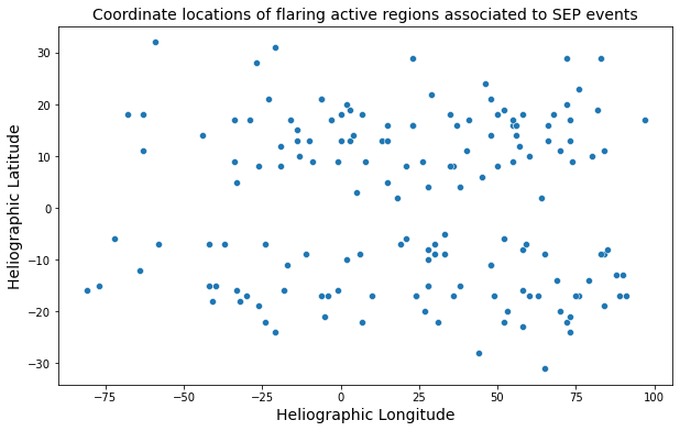
The magnetic connectivity between the Sun and Earth is strong over the western hemisphere on the Sun and until \(-30^0\) toward the eastern side. In the figure above, it can be noticed that while most events occur in the magnetically well-connected western regions on the Sun, there are ~20% of the total events originating from the eastern hemisphere, solar limbs and farside (behind the Sun).
Furthermore, there is a spread of flaring active reagion locations across the solar hemisphere. It is interesting to observe particles reach Earth in the interplanetary magnetic fields that are several tens of degrees beyond the Sun-Earth connecting regions of the Parker spiral.
Impacts: Dosage rate#
An important effect of SEP events is the dosage rate on astronauts and electronic equipment [8], [9]. The histogram shows the proton flux levels measured in particle flux units (pfu) according to the NOAA solar radiation storm-scale. The figure below (Credit: NOAA-SWPC, [https://www.swpc.noaa.gov/noaa-scales-explanation]), describing the S-scale with reference the effects of the SEP event levels.

## Plotting Distribution of bins defined on gsep_pf_gt10_bins
fig, x = plt.subplots(figsize=(8,6))

sns.countplot(x="gsep_pf_gt10_bins", data=sep_ar_data,color='blue',saturation=0.9,order=["S1","S2","S3","S4"])
plt.xlabel('Scale', fontsize=14);
plt.ylabel('Number of events', fontsize=14);
plt.title('Distribution of large SEP events according to the NOAA S-scale', fontsize=14)
Text(0.5, 1.0, 'Distribution of large SEP events according to the NOAA S-scale')
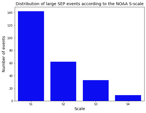
The base scale (S1) is at 10 pfu and continues to logarithmically increase from the previous scale. The number of events in the S1 category is high indicating minor effects. However, there are several events measured in the higher scales that could impact biologically and technologically in space.
Interestingly, we do not observe any S5 events in the last three solar cycles based on our dataset. Events in that scale are extremely rare and we are only counting the things that came towards Earth.
Historical fact: The GOES proton fluxes were observed at S4 levels for 12 hours on 29-Oct-2003 (the famous Halloween storm) [10].
SEP Event Occurrence Probability Modeling#
def groupby_bins(data_df,col_1,col_2,col_agg):

    '''
    Function to compute the aggregated counts of SEP events for each pair of
    defined lon & lat bins.

    Inputs :
    data_df - Merged dataframe
    col_1- First column used for grouping ( lat bins)
    col_2 -Second column used for grouping ( lon bins)
    col_agg- The column on which aggregation is done (sep_index)

    Returns :
    grop_bin_df- A dataframe which stores distinct pairs of bins and the count of SEP events, respectively.

    '''


    groups = data_df.groupby([col_1, col_2])
    grop_bin_df=pd.DataFrame()
    ## Counting Number of SEPs for each pair of the spatial bins
    grop_bin_df[col_agg+'_count']=groups[col_agg].count()

    grop_bin_df=grop_bin_df.reset_index()
    return grop_bin_df
## Calling function to group dataframe. For 12 lon_bins & 10 lat bins, we got 120 different pairs

SEP_bin_df=groupby_bins(sep_ar_data,"AR_Lat_bin_names", "AR_Lon_bin_names","sep_index")
SEP_bin_df.head(3)
| AR_Lat_bin_names | AR_Lon_bin_names | sep_index_count | |
|---|---|---|---|
| 0 | (-90.001, -72.0] | (-180.001, -90.0] | 0 |
| 1 | (-90.001, -72.0] | (-90.0, -72.0] | 0 |
| 2 | (-90.001, -72.0] | (-72.0, -54.0] | 0 |
def load_clean_halo_cme(data_hcme,bins):

    '''
     Function to load and clean the Halo CME data.

     Input :
     -data_hcme : A pandas dataframe extracted in the data loading stage from the url:
     https://cdaw.gsfc.nasa.gov/CME_list/halo/halo.html

     - bins : A tuple which will consist list for two binning strategies.


     Returns:
     A dataframe consisting of Halo CME data.

    '''


    table_MN = data_hcme
    ## Removing source location values consisting "Backside" or ends with b or having --
    patternDel = "Backside*|.*b|--.*"
    filter = table_MN[1]['Source Location'].str.contains(patternDel)
    Halo_df=table_MN[1][~filter]

    ## Formatting columns of dataframe
    df_split1=Halo_df['Source Location'].str.split('[NSEW?]|>', expand=True)
    df_split1.columns = ['g1', "Lat","Long",'g2']
    ## Direction string for the coordinates
    df_split2=Halo_df['Source Location'].str.split('\d+', expand=True)
    df_split2.columns = ["Lat_direction", "Long_direction","g3"]

    ## Converting coordinates values to numerical data types.
    ## Multiplying the coordinates with -1 if the direction is either S or E
    cordinates_df=pd.concat([df_split1,df_split2],axis=1)
    cordinates_df["Lat"]=pd.to_numeric(cordinates_df["Lat"])
    cordinates_df["Long"]=pd.to_numeric(cordinates_df["Long"])
    cordinates_df["Lat"]=np.where(cordinates_df['Lat_direction'] == 'S',
                                           cordinates_df['Lat'] * -1,
                                           cordinates_df['Lat'])
    cordinates_df["Long"]=np.where(cordinates_df['Long_direction'] == 'E',
                                           cordinates_df['Long'] * -1,
                                           cordinates_df['Long'])

    HCME_df=pd.concat([Halo_df,cordinates_df[['Lat',"Long"]]],axis=1)

    ## Longitude coordinates ranging outside [-180,180] will be transformed to the correct values
    ## For example: -184 will be converted to 176, which will now be on the east direction.
    ## All values ranging outside the range [-180,180] will be shifted to the other direction using the transformation
    HCME_df["Long"]=np.where(HCME_df["Long"]<-180,HCME_df["Long"]+360,HCME_df["Long"] )
    HCME_df["Long"]=np.where(HCME_df["Long"]>180,HCME_df["Long"]-360,HCME_df["Long"] )


    ## Binning the dataframe
    HCME_df['HCME_Lat_bin_names'] = pd.cut(HCME_df['Lat'], bins[1],include_lowest=True)
    HCME_df['HCME_Lon_bin_names'] = pd.cut(HCME_df['Long'], bins[0],include_lowest=True)
    HCME_df=HCME_df.reset_index()
    HCME_df.rename(columns = {'index':'HCME_index'}, inplace = True)

    return HCME_df
## Calling function to get clean halo CME dataframe

HCME_df=load_clean_halo_cme(data_hcme,bins)
## Calling function to group dataframe. For 12 lon bins & 10 lat bins, we get 120 different pairs.

HCME_bin_df=groupby_bins(HCME_df,'HCME_Lat_bin_names','HCME_Lon_bin_names','HCME_index')
def laplacian_prob_smoothing(SEP_bin_df,HCME_bin_df,k=1):
    '''
    Function to merge both SEP grids dataframe and Halo CME dataframe.
    On the merged dataframe, the conditional probabilities of occurence of SEPs and Halo CMEs in spatial grids
    are computed. The probabilities are then distributed using Laplacian smoothing.

    Laplacian smoothing--->              (count(A) +K)
                            P(A|B)=   ------------------   ; where K is a constant
                                      count(B)+K*Domain{X}

    Inputs :
    SEP_bin_df - Grouped dataframe for SEP
    HCME_bin_df - Grouped dataframe for Halo CME data
    k- An integer for laplacian smoothing

    Returns :
    A merged data frame with laplacian smoothed probabilities

    '''
    ## Merging the two dataframe on the active region spatial bins created for SEP data and Halo CME.
    cond_prob_df=SEP_bin_df.merge(HCME_bin_df,how='inner',
                              left_on=['AR_Lat_bin_names','AR_Lon_bin_names'],
                                  right_on = ['HCME_Lat_bin_names','HCME_Lon_bin_names'])
    ## Computed laplacian smoothing to distribute probabilities among zero probabilities
    cond_prob_df["Laplacian_smoothing"]=(cond_prob_df["sep_index_count"] + k) / (cond_prob_df["HCME_index_count"] + (k*cond_prob_df.shape[0]))
    return cond_prob_df
## Calling the function

lap_prob_df=laplacian_prob_smoothing(SEP_bin_df,HCME_bin_df,k=1)
## Making copy of the dataframe

final_lap_df=lap_prob_df.copy()
## Splitting the lat bins into two atomic values; start and end of the bins

final_lap_df[['Lat_bin_start','Lat_bin_end']]=final_lap_df['AR_Lat_bin_names'].astype(str).str.split(',',expand=True)
final_lap_df["Lat_bin_start"]=final_lap_df["Lat_bin_start"].str[1:]
final_lap_df["Lat_bin_end"]=final_lap_df["Lat_bin_end"].str[:-1]
## Splitting the lon bins into two atomic values; start and end of the bins

final_lap_df[['Lon_bin_start','Lon_bin_end']]=final_lap_df['AR_Lon_bin_names'].astype(str).str.split(',',expand=True)
final_lap_df["Lon_bin_start"]=final_lap_df["Lon_bin_start"].str[1:]
final_lap_df["Lon_bin_end"]=final_lap_df["Lon_bin_end"].str[:-1]

final_lap_df=final_lap_df[["Lon_bin_start","Lon_bin_end","Lat_bin_start","Lat_bin_end","Laplacian_smoothing"]]

final_lap_df.head(3)
| Lon_bin_start | Lon_bin_end | Lat_bin_start | Lat_bin_end | Laplacian_smoothing | |
|---|---|---|---|---|---|
| 0 | -180.001 | -90.0 | -90.001 | -72.0 | 0.008333 |
| 1 | -90.0 | -72.0 | -90.001 | -72.0 | 0.008333 |
| 2 | -72.0 | -54.0 | -90.001 | -72.0 | 0.008333 |
## Pivot table on spatial bins. Each element of the pivot table will denote the laplacian smoothing calculated for
## the respective pairs of spatial bins

piv = pd.pivot_table(lap_prob_df, values="Laplacian_smoothing",index=["AR_Lat_bin_names"], columns=["AR_Lon_bin_names"], fill_value=0)
piv
| AR_Lon_bin_names | (-180.001, -90.0] | (-90.0, -72.0] | (-72.0, -54.0] | (-54.0, -36.0] | (-36.0, -18.0] | (-18.0, 0.0] | (0.0, 18.0] | (18.0, 36.0] | (36.0, 54.0] | (54.0, 72.0] | (72.0, 90.0] | (90.0, 180.0] |
|---|---|---|---|---|---|---|---|---|---|---|---|---|
| AR_Lat_bin_names | ||||||||||||
| (-90.001, -72.0] | 0.008333 | 0.008333 | 0.008333 | 0.008333 | 0.008333 | 0.008333 | 0.008333 | 0.008333 | 0.008333 | 0.008333 | 0.008333 | 0.008333 |
| (-72.0, -54.0] | 0.008333 | 0.008333 | 0.008333 | 0.008333 | 0.008264 | 0.008333 | 0.008333 | 0.008333 | 0.008333 | 0.008333 | 0.008333 | 0.008333 |
| (-54.0, -36.0] | 0.008333 | 0.008333 | 0.008333 | 0.008333 | 0.008333 | 0.008197 | 0.008264 | 0.008264 | 0.008333 | 0.008333 | 0.008333 | 0.008197 |
| (-36.0, -18.0] | 0.007299 | 0.008264 | 0.008065 | 0.016129 | 0.038462 | 0.015152 | 0.015267 | 0.023810 | 0.032000 | 0.040984 | 0.032000 | 0.007463 |
| (-18.0, 0.0] | 0.006579 | 0.031496 | 0.023256 | 0.038168 | 0.037594 | 0.042857 | 0.028777 | 0.099291 | 0.047619 | 0.062016 | 0.078125 | 0.014184 |
| (0.0, 18.0] | 0.006757 | 0.007752 | 0.031496 | 0.015385 | 0.058394 | 0.078014 | 0.074324 | 0.062069 | 0.069767 | 0.115385 | 0.047619 | 0.013245 |
| (18.0, 36.0] | 0.007752 | 0.008264 | 0.016129 | 0.008130 | 0.031496 | 0.022901 | 0.022388 | 0.023810 | 0.031746 | 0.024194 | 0.032787 | 0.008197 |
| (36.0, 54.0] | 0.008333 | 0.008264 | 0.008333 | 0.008333 | 0.008333 | 0.008333 | 0.008130 | 0.008333 | 0.008333 | 0.008333 | 0.008197 | 0.008333 |
| (54.0, 72.0] | 0.008333 | 0.008333 | 0.008333 | 0.008333 | 0.008333 | 0.008333 | 0.008333 | 0.008333 | 0.008333 | 0.008333 | 0.008333 | 0.008333 |
| (72.0, 90.0] | 0.008333 | 0.008333 | 0.008333 | 0.008333 | 0.008333 | 0.008333 | 0.008333 | 0.008333 | 0.008333 | 0.008333 | 0.008333 | 0.008333 |
#plot pivot table as heatmap using seaborn
fig, x = plt.subplots(figsize=(8,8))
pl = sns.heatmap(piv, square=True,ax=x,cbar_kws={"shrink": 0.5})
plt.setp( pl.xaxis.get_majorticklabels(), rotation=90)
plt.xlabel("Latitude bins",fontsize=14)
plt.ylabel("Longitude bins",fontsize=14)
plt.title("Active Region bins in Heliographic Coordinates", fontsize=14)
plt.tight_layout()
plt.show()
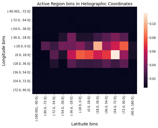
The probability of occurrence model satisfactorily reflects the observational evidences of SEP event association to the source active regions. From the heat map shown above, we can notice the higher probability of magnetic connectivity of eruptive regions from central to the western hemisphere of the Sun.
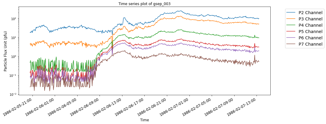
Part Two - Time series visualizations#
The integral proton fluxes from GOES satellites are downloaded from the NOAA server [https://satdat.ngdc.noaa.gov/sem/goes/data/avg/] and sorted for reliable missions. Two GOES missions making parallel observations are denoted as primary and secondary. The differences in their measurements occur because of the geomagnetic cut-off [7]. Hence, we understand the possible variations by visually inspecting the time series data and sorting them into reliable missions. Furthermore, the proton flux data is smoothed and imputed across all missions. Then, a subset of time series is obtained for each SEP event based on the event start and end time as reported in the GSEP catalog. We maintain an observation window of 12 hours before the event onset. These subsets or time series slices are stored on Harvard Dataverse.
GSEP Slices#
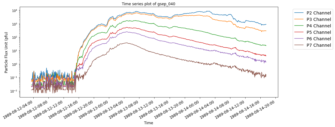
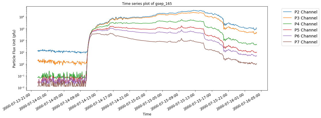
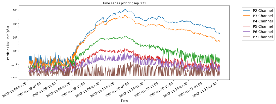
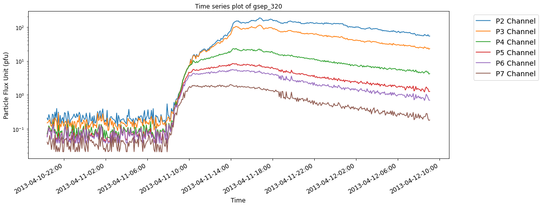
SEP events are theoretically classified as impulsive and gradual events based on the nature of the temporal evolution of particles originating from the Sun. Impulsive events have beam-like proton flux profiles while gradual events are observed as slowly decreasing in proton flux, lasting longer and posing much bigger threat of radiation exposure to astronauts.
The below time series plots show typical examples of SEP events with reference to their source eruptions. For illustrative purposes, two events each from the last three solar cycles are selected from the GSEP list, respectively. The indeces of the events are gsep_003, gsep_040, gsep_165, gsep_231, gsep_320 and gsep_340
def file_name_(x):
    '''
    Function to perform string manipulation to create time series slice filename convention

    Inputs :
    x - A string

    Returns:
    filename - String in the format yyyy-mm-dd_HH-MM.csv
    '''
    x_temp=x[:-3]
    filename=x_temp.replace(":","-")+".csv"
    return filename
def loading_ts_from_tar(t22,t23,t24,filename):

    '''
    Function to load time series slice inside tar files into a dataframe

    Inputs :
    t22 - string for gsep_sc22 zip file
    t23 - string for gsep_sc23 zip file
    t24 - string for gsep_sc24 zip file
    filename - string of the filename to serach for

    Returns :
     A data frame corresponding to time series slice. Note: It will return an empty dataframe if filename is
     not found inside any of the tar
    '''
    ## Opening tar objects
    tar1 = tarfile.open(t22)
    tar2 = tarfile.open(t23)
    tar3 = tarfile.open(t24)

    ## Storing CSV files inside list
    csv_files_1 = [f.name for f in tar1.getmembers() if f.name.endswith('.csv')]
    csv_files_2 = [f.name for f in tar2.getmembers() if f.name.endswith('.csv')]
    csv_files_3 = [f.name for f in tar3.getmembers() if f.name.endswith('.csv')]

    data=pd.DataFrame()

    ## Searching file in gsep_sc22 zip
    for index, value in enumerate(csv_files_1):
            if filename in value:
                csv_contents = tar1.extractfile(value).read()
                df = pd.read_csv(io.BytesIO(csv_contents), encoding='utf8')
                data=df

    ## Searching file in gsep_sc23 zip
    for index, value in enumerate(csv_files_2):
            if filename in value:
                csv_contents = tar2.extractfile(value).read()
                df = pd.read_csv(io.BytesIO(csv_contents), encoding='utf8')
                data=df

    ## Searching file in gsep_sc24 zip
    for index, value in enumerate(csv_files_3):
            if filename in value:
                csv_contents = tar3.extractfile(value).read()
                df = pd.read_csv(io.BytesIO(csv_contents), encoding='utf8')
                data=df

    return data
def time_series_slice_df(data_df, sep_index):

    '''
    Function to read sep_index and merged sep_ar_data and return the time series slice for
    the respective index value

    Inputs :
    data_df - A dataframe - sep_ar_data dataframe
    sep_index - A string ; for example gsep_003

    Returns :
    time_series_df- Time series slice for sep_index
    '''
    ## tar files downloaded from the GSEP dataset available on Harvard Dataverse
    t22="gsep_sc22.tar.gz"
    t23="gsep_sc23.tar.gz"
    t24="gsep_sc24.tar.gz"

    ## string manipulation to convert slice_start column in metadata ti file format
    data_df['slice_start_temp']=data_df['slice_start'].replace(" ","_",regex=True)

    ## This column will store the string in the conventions of csv files; calling function using apply()
    data_df["filename"]=data_df['slice_start_temp'].apply(file_name_)

    ## Extracting filename as a string
    ts_file=data_df.loc[data_df['sep_index']==sep_index]["filename"].to_list()[0]

    ## Calling function to get time series for the sep index
    time_series_df=loading_ts_from_tar(t22,t23,t24,ts_file)

    return time_series_df
def visualize_ts(time_series_df,sep_ar_data,sep_index):

    '''
    Function to visualize the time series for a given SEP event

    Inputs:
    -time_series_df : A pandas dataframe which consist time series slice
    -sep_ar_data : A pandas dataframe that has meta data information
    -sep_index : A string for sep_index

    Returns:
    Time series plot
    '''

    ## Extracting SEP event onset and peak time,
    single_sep_data=sep_ar_data.loc[sep_ar_data['sep_index']==sep_index]
    sep_start_time=(pd.to_datetime(single_sep_data["slice_start"])+pd.DateOffset(hours=12)).to_list()[0] ## slice time +12h
    sep_max_time=pd.to_datetime(single_sep_data["gsep_max_time"]).to_list()[0]

    ## Extracting flare metadata,
    flare_start_time=pd.to_datetime(single_sep_data["fl_start_time"]).to_list()[0]
    fl_goes_class=str(single_sep_data["fl_goes_class"].to_list()[0])

    ## Extracting CME launch time from GSEP metadata
    cme_launch_time=pd.to_datetime(single_sep_data["cme_launch_time"]).to_list()[0]
    cme_vel=str(single_sep_data["lasco_linear_speed"].to_list()[0])
    cme_width=str(single_sep_data["lasco_cme_width"].to_list()[0])
    cme_details= '('+"v:"+" "+cme_vel+","+"w:"+cme_width+')'


    ## Figusre size
    plt.figure(figsize=(15, 6))

    ## Plot components
    plt.xlabel("Time",fontsize=12)
    plt.ylabel("Particle Flux Unit (pfu)",fontsize=12)
    plt.title("Time series plot of" +" "+ sep_index ,fontsize=12)
    plt.grid(False)

    ## Visualizing P2-P7 proton channels
    plt.plot(time_series_df["p2_flux_ic"],label='P2 Channel')
    plt.plot(time_series_df["p3_flux_ic"],label='P3 Channel')
    plt.plot(time_series_df["p4_flux_ic"],label='P4 Channel')
    plt.plot(time_series_df["p5_flux_ic"],label='P5 Channel')
    plt.plot(time_series_df["p6_flux_ic"],label='P6 Channel')
    plt.plot(time_series_df["p7_flux_ic"],label='P7 Channel')
    ax = plt.gca()
    ax.set_yscale('log') ## Logrithmic scale -y axis

    ## Defining frequency and format of x tick labels
    ax.xaxis.set_major_locator(mdates.HourLocator(interval=4))
    ax.xaxis.set_major_formatter(mdates.DateFormatter('%Y-%m-%d-%H:%M'))

    ## Plotting vertical lines of extracted meta data information.
    ##If any of the profile is not available, will not plot the vertical lines. Handling this through try & pass
    try:
        ax.axvline(sep_start_time, color='red', linestyle='--', label='Event Onset',alpha=15)
    except:
        pass
    try :
        ax.axvline(sep_max_time, color='black', linestyle='--', label='Event Peak',alpha=15)
    except:
        pass
    try:
        ax.axvline(flare_start_time, color='green', linestyle='--',
                   label='Flare Onset'+' '+'('+fl_goes_class+')', alpha=15)
    except:
        pass
    try :
        ax.axvline(cme_launch_time, color='yellow', linestyle='--',
                   label='CME Launch'+' '+cme_details,alpha=15)
    except:
        pass
    plt.gcf().autofmt_xdate() # Rotation
    plt.legend(bbox_to_anchor=(1.05, 1), loc='upper left',fontsize=14)
    plt.xticks(fontsize=12)
    plt.show()
def plot_vis(sep_ar_data,sep_index):

    '''
    Function to call the visualization module for any
    given SEP Event

    Inputs:
    - sep_ar_data : Pandas dataframe that has metadata information merged with NOAA active region information
    -sep_index : String for sep_index

    Outputs:
    Plot for given SEP Index

    '''

    time_series_df=time_series_slice_df(sep_ar_data,sep_index) # Function call to get time series
    time_series_df["time_stamp"]=pd.to_datetime(time_series_df["time_stamp"])
    time_series_df=time_series_df.set_index('time_stamp')
    visualize_ts(time_series_df,sep_ar_data,sep_index)
## Calling the plotting function on the event index gsep_003

plot_vis(sep_ar_data,'gsep_003')
## Calling the plotting function on the event index gsep_040

plot_vis(sep_ar_data,'gsep_040')
## Calling the plotting function on the event index gsep_165

plot_vis(sep_ar_data,'gsep_165')
## Calling the plotting function on the event index gsep_231

plot_vis(sep_ar_data,'gsep_231')
## Calling the plotting function on the event index gsep_320

plot_vis(sep_ar_data,'gsep_320')
## Calling the plotting function on the event index gsep_340

plot_vis(sep_ar_data,'gsep_340')
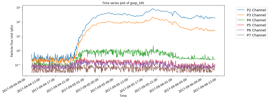
We believe this tool will be a useful helper utility for visual analytics of SEP events, specifically for understanding the statistical distributions of time differences between SEP start times and associated flare/CME occurrences.
References#
Athanasios Papaioannou, Ingmar Sandberg, Anastasios Anastasiadis, Athanasios Kouloumvakos, Manolis K. Georgoulis, Kostas Tziotziou, Georgia Tsiropoula, Piers Jiggens and Alain Hilgers, “Solar flares, coronal mass ejections and solar energetic particle event characteristics.” J. Space Weather Space Clim., 6 (2016) A42, DOI: https://doi.org/10.1051/swsc/2016035
CDAW Major SEP Events List, https://cdaw.gsfc.nasa.gov/CME_list/sepe/
S. Rotti, B. Aydin, M. Georgoulis, and P. Martens, “GSEP Dataset.” Harvard Dataverse, 2022. doi: 10.7910/DVN/DZYLHK.
Reames, D.V. The Two Sources of Solar Energetic Particles. Space Sci Rev 175, 53–92 (2013). https://doi.org/10.1007/s11214-013-9958-9
Anastasiadis Anastasios, Lario David, Papaioannou Athanasios, Kouloumvakos Athanasios and Vourlidas Angelos 2019 Solar energetic particles in the inner heliosphere: status and open questionsPhil. Trans. R. Soc. A.3772018010020180100 http://doi.org/10.1098/rsta.2018.0100
Terrance Onsager, Richard Grubb, Joseph Kunches, Lorne Matheson, David Speich, Ron W. Zwickl, and Herb Sauer “Operational uses of the GOES energetic particle detectors”, Proc. SPIE 2812, GOES-8 and Beyond, (18 October 1996); https://doi.org/10.1117/12.254075
Rodriguez, J.V., Krosschell, J.C. and Green, J.C., 2014. Intercalibration of GOES 8–15 solar proton detectors. Space Weather, 12(1), pp.92-109. https://doi.org/10.1002/2013SW000996
Pulkkinen, T. Space Weather: Terrestrial Perspective. Living Rev. Sol. Phys. 4, 1 (2007). https://doi.org/10.12942/lrsp-2007-1
Jiggens, P; Clavie, C; Evans, H; O’Brien, TP; Witasse, O; Mishev, AL; et al. (2019): In Situ Data and Effect Correlation During September 2017 Solar Particle Event. University of Leicester. Journal contribution. https://hdl.handle.net/2381/11536293.v1
Intense Space Weather Storms, October 19 - November 7, 2003, Service Assessment https://www.weather.gov/media/publications/assessments/SWstorms_assessment.pdf