Jupyter Notebooks as a bridge to the MagIC Database and Open Science#

Author(s)#

Author1 = {“name”: “Lisa Tauxe”, “affiliation”: “Scripps Institution of Oceanography”, “email”: “ltauxe@ucsd.edu”, “orcid”: “0000-0002-4837-8200”}
Author2 = {“name”: “Rupert Minnett”, “affiliation”: “Oregon State University”, “email”: “rminnett@earthref.org”, “orcid”: “0000-0002-9000-2100”}
Author3 = {“name”: “Nick Jarboe”, “affiliation”: “Oregon State University”, “email”: “njarboe@earthref.org”, “orcid”: “0000-0003-1465-9394”}
Author4 = {“name”: “Catherine Constable”, “affiliation”: “Scripps Institution of Oceanography”, “email”: “cconstable@ucsd.edu”, “orcid”: “0000-0003-4534-4977”}
Author5 = {“name”: “Anthony Koppers”, “affiliation”: “Oregon State University, “email”: “Oregon State University, “orcid”: “0000-0002-8136-5372”}

Purpose#

This notebook demonstrates how to access data in the MagIC open-source database at https://earthref.org/MagIC. MagIC is the first of a set of data repositories created by the EarthCube-funded project FIESTA. The MagIC Database (Magnetics Information Consortium) allows magnetic measurement data of rocks and archaeological artifacts to be more Findable, Accessible, Interoperable, and Re-usable. The MagIC Data Model governs the dataset contributions in the MagIC Database and is fully described here: https://earthref.org/MagIC/data-models/3.0. PmagPy is a cross-platform and open-source software package with Python functions written for the analysis of paleomagnetic and rock magnetic data, including tools that facilitate uploading, downloading and (re)interpretion of data in the MagIC Database. It is intended to make the uploading of paleomagnetic data into MagIC straight-forward as MagIC data tables are created as part of normal data analysis and these can be uploaded to MagIC using the EarthCube-unded FIESTA API https://api.earthref.org within a Jupyter notebook or through the MagIC website itself.

Overview of the MagIC database#

Figure 1 shows the basic workflow of a typical paleomagnetic project from sampling in the field to contributing to the MagIC Database. Samples are taken in the field, and prepared into specimens, which then get measured. The measurements can be made on many different measurements and converted into a single, standard (MagIC) format which can then be operated on by an open-source software package, PmagPy to visualize and interpret the data. The measurement data and interpretations can be compiled into a hierarchy of MagIC data tables and then uploaded into the MagIC database.

Figure 1: Workflow of a typical paleomagnetic project (from Tauxe et al., 2016; doi:10.1002/2016GC006307)

The MagIC Data Model is built with the hierarchical structure typical of paleomagnetism whereby samples are taken in the field from “sites”, which are considered homogeneous with respect to the magnetic property being measured (for example a lava flow or sedimentary horizon). Sites can be grouped into “locations” which can be stratigraphic sections, drill cores, or regions. The links between specimens, samples, sites, and locations are specified in the various data tables in the MagIC data format.

Each contribution in the database is associated with a publication via the DOI. There are nine data tables:

contribution: metadata of the associated publication.
locations: metadata for locations, which are groups of sites (e.g., stratigraphic section, region, etc.)
sites: metadata and derived data at the site level (units with a common expectation)
samples: metadata and derived data at the sample level.
specimens: metadata and derived data at the specimen level.
measurements: metadata and measurements made on specimens from which all other data are derived
criteria: criteria by which data are deemed acceptable
ages: ages and metadata for sites/samples/specimens
images: associated images and plots.

Only the contribution and location tables are required for a given study, but others can be used if desired. The most useful datasets include the measurements table and the full hierarchy of data tables.

Overview of the PmagPy software package#

PmagPy is a software package with over 1000 functions grouped into several modules that provide data analysis tools for visualizing and interpreting many different kinds of data including those in the MagIC format. It can be accessed through https://github.com/PmagPy/PmagPy and downloaded onto a personal computer following instructions in the PmagPy cookbook https://earthref.org/PmagPy/cookbook/. There are many notebooks in the PmagPy software package which can also be run without installation through the website: https://jupyterhub.earthref.org after creating a personal user’s space and running a simple Jupyter notebook (PmagPy_online setup).

Functions as simple as calculating the expected direction at a given latitude to those as complicated as interpreting paleointensity data are available. Most functions for making such calculations are grouped into the pmag module. Functions for making specialized plots are grouped into the pmagplotlib module. Functions specifically designed for use within Jupyter notebooks are grouped in the ipmag module. There are also a number of command line programs that allow similar data analysis to be performed as in the notebooks. Finally, there are several Graphical User Interfaces (GUIs) that, when installed on a personal computer aid in interpretation and data analysis, call the many functions in the PmagPy package. This notebook focuses on the use of Jupyter Notebooks for using the PmagPy functions.

Use of PmagPy from within a Jupyter notebook#

Notebooks such as this one can be used to call PmagPy functions. They can be used to convert data from laboratory formats into the MagIC format and produce many of the plots and make the calculations required in paleomagnetic projects.

Data can be accessed either through a web browser or through the FIESTA API queries, the most direct of which connects a dataset to the DOI of the publication using Python code that is part of the PmagPy software package. Data can therefore be downloaded, unpacked, re-analyzed or imaged and then repackaged and uploaded back into a private workspace of the user. Jupyter notebooks can then be attached to a new publication and serve as important supplemental material for publication, making the data and the analysis thereof transparent and reproducible. We will illustrate the use of Jupyter notebooks in connection with FAIR data practices in the rock and paleomagnetic world.

Technical contributions#

Paleomagnetic data published on the MagIC website and linked to a DOI can be downloaded from the database using the FIESTA API.
The PmagPy python software package imported in the notebook can be used to unpack and re-analyze data in the database to reproduce results, demonstrating the benefits of FAIR principles.

Methodology#

import useful Python modules
import the PmagPy software package
download a dataset from MagIC using the FIESTA API through PmagPy
re-analyze the data using PmagPy plotting and analysis functions

Results#

This notebook illustrates how open-source databases can be accessed and used to further the goals of open science.

Funding#

Award1 = {“agency”: “US National Science Foundation”, “award_code”: “1822336”, “award_URL”: “https://www.nsf.gov/awardsearch/showAward?AWD_ID=1822336”}
Award2 = {“agency”: “US National Science Foundation”, “award_code”: “2126298”, “award_URL”: “https://www.nsf.gov/awardsearch/showAward?AWD_ID=2126298”}

Keywords#

keywords=[“FAIR”, “Open Science”, “MagIC database”, “PmagPy software package”, “paleomagnetism”]

Citation#

Tauxe et al., 2022, Jupyter Notebooks as a bridge to the MagIC Database and Open Science, 2022 EarthCube Annual Meeting. Accessed XX/XX/XXXX at https://github.com/PmagPy/2022_Tauxe-et-al_MagIC-Database-and-Open-Science

Acknowledgements#

We thank members of the MagIC/FIESTA database team Nick Swanson-Hysell and Christeanne Santos for help in maintaining the PmagPy software package. We also thank EarthCube for providing support for the further development of PmagPy and MagIC under the umbrella of the FIESTA project, meant to expand database design beyond MagIC into other geoscience domains.

The template is licensed under a Creative Commons Attribution 4.0 International License.

Setup#

Access of the notebook:#

Using Binder#

This notebook can be run by launching Binder from the GitHub repository.

Go to https://github.com/earthcube2022/ec22_tauxe_etal.git and click on Binder label at the top of the README.md file.
Once the dependencies are installed, JupyterLab loads, and the notebook opens, the cells in the notebook can be executed and edited as needed.

Using jupyterhub#

The Binder version does not allow uploading of user’s own data and is therefore useful only for demonstration purposes. However, this notebook is also included in the PmagPy software package which can be installed on a personal and downloaded onto a personal computer following instructions in the PmagPy cookbook https://earthref.org/PmagPy/cookbook/or run without installation through the website: https://jupyterhub.earthref.org.

Library import#

Import all the required Python libraries.

# This allows you to make matplotlib plots inside the notebook
%matplotlib inline
# Import packages
import pandas as pd # and  Pandas for data wrangling
import os # some useful operating system functions
from IPython.display import Image

Local library import#

import the special PmagPy and mapping modules
create a directory for use in this notebook

# Import PmagPy modules
import pmagpy.pmag as pmag
import pmagpy.pmagplotlib as pmagplotlib
import pmagpy.ipmag as ipmag

dirs=os.listdir() # get a list of directories in this one
if 'MagIC_for_earthcube' not in dirs:
    os.mkdir("MagIC_for_earthcube")

Parameter definitions#

after installation of PmagPy software, set up the directory structure for this notebook
Define path, desired DOI for downloading data from MagIC and a placeholder filename.

dir_path='MagIC_for_earthcube' # set the path to the working directory
reference_doi='10.1029/2019GC008479' # Behar et al. (2019)
magic_contribution='magic_contribution.txt' # temporary name for contribution prior to unpacking

Data import#

Retrieve all the required data for the analysis.

We will be using the data from this reference:

Behar, N., Shaar, R., Tauxe, L., Asefaw, H., Ebert, Y., Heimann, A., Koppers, A.A.P., and Ron, H., Paleomagnetic study of the Plio-Pleistocene Golan Heights volcanic field, Israel: confirmation of the GAD field hypothesis, Geophys., Geochem. Geosyst., 20, doi: 10.1029/2019GC008479, 2019.

The purpose of that paper was to provide new data relating to the geomagnetic field over the last few million years. The Plain Language Summary stated:

“Since the early days of paleomagnetic research, it has been inferred that the time‐averaged structure of the field is a geocentric axial dipole (GAD)—equivalent to a field generated by a dipole at the center of the Earth aligned with its rotation axis. This so‐called GAD hypothesis is fundamental in paleomagnetism and is the basis for plate tectonic reconstructions. However, recent studies have suggested persistent departures from a GAD structure, manifested as an anomaly in the inclination angle of the field in northern hemispheric low to middle latitudes. To address this problem, we analyzed 91 basaltic lava flows from the Golan Heights volcanic plateau in Israel (32–33°N), spanning the past 5 Myr. As each basaltic flow captured the direction of the ambient magnetic field when it cooled, these flows provide us information about the averaged direction of the ancient geomagnetic field. Our results show that the averaged field in the Golan Heights is in agreement with a GAD structure. We also show that if we reanalyze the global paleomagnetic data from lava flows spanning the past 10 Myr using stricter selection criteria and a different inclination anomaly calculation method, the data do not support a global non‐GAD field.”

In this notebook, we will reproduce a few of the key diagrams in the paper.

Steps for data import:

create a directory to put downloaded data
download the data from the database using the reference DOI
move the data to the directory
unpack the data into MagIC formatted tab-delimited files.

For help on all functions use: help(ModuleName.FunctionName)

example:

help(ipmag.download_magic_from_doi)

Help on function download_magic_from_doi in module pmagpy.ipmag:

download_magic_from_doi(doi)
    Download a public contribution matching the provided DOI
    from earthref.org/MagIC.
    
    Parameters
    ----------
    doi : str
        DOI for a MagIC
    
    Returns
    ---------
    result : bool
    message : str
        Error message if download didn't succeed

ipmag.download_magic_from_doi(reference_doi)
os.rename(magic_contribution, dir_path+'/'+magic_contribution)
ipmag.download_magic(magic_contribution,dir_path=dir_path,print_progress=False)

16961/magic_contribution_16961.txt extracted to magic_contribution.txt 

records written to file  /Users/ltauxe/PmagPy/MagIC_for_earthcube/contribution.txt
records written to file  /Users/ltauxe/PmagPy/MagIC_for_earthcube/locations.txt
records written to file  /Users/ltauxe/PmagPy/MagIC_for_earthcube/sites.txt
records written to file  /Users/ltauxe/PmagPy/MagIC_for_earthcube/samples.txt
records written to file  /Users/ltauxe/PmagPy/MagIC_for_earthcube/specimens.txt
records written to file  /Users/ltauxe/PmagPy/MagIC_for_earthcube/measurements.txt
records written to file  /Users/ltauxe/PmagPy/MagIC_for_earthcube/criteria.txt
records written to file  /Users/ltauxe/PmagPy/MagIC_for_earthcube/ages.txt

True

Data processing and analysis#

We will look at three examples of reuse of the data from our study. The first will make an equal area projection of all the directions found in the study. Paleomagnetists often deal with directional data (Figures 2a,b) and like other Earth Science disciplines (e.g., structural geology) plot directions that are inherently three-dimensional on a 2-D projection (Figure 2c). Plotted in this way one can assess whether the directions behave as one might expect from secular variation of the field. For example, in our second plot, we will check whether two sets of directions from the two polarities, normal (as in the present field) and reverse (opposite), are antipodal.

Figure 2: a) Lines of flux of the geomagnetic field of 2005. At point \(P\) the horizontal component of the field \(B_H\), is directed toward the magnetic north (with a deviation known as declination, \(D\)). The vertical component \(B_V\) is directed down and the field makes an angle \(I\) with the horizontal, known as the inclination. b) Components of the geomagnetic field vector \(B\). c) Construction of an equal area projection for a point \(P\) corresponding to a \(D\) of 40\(^{\circ}\) and an \(I\) of 35\(^{\circ}\). d) Transformation of a direction measured at location \(S\) to a virtual geomagnetic pole (VGP). Figure modified from https://earthref.org/MagIC/books/Tauxe/Essentials/ and references therein.

In the third plot, we will look at the directional data after transformation to virtual geomagnetic pole positions (Figure 2d). These we will plot on an orthorhombic projection with the reverse poles (negative latitudes) flipped to their antipodes.

For more information on Paleomagnetism, check out the open-source textbook hosted by MagIC at: https://earthref.org/MagIC/books/Tauxe/Essentials/.

MagIC formatted files#

MagIC text files all have the delimiter (tab) and the type of table in the first line and the column headers in the second line. For details on the column headers in each data table, see the current MagIC database model definitions here: https://earthref.org/MagIC/data-models/3.0

To read in the site level data into a Pandas DataFrame we specify that the file is tab-delimited with the sep argument and that the header is in the second row (remember that Pandas starts counting at zero). Then we will look at the first few lines using the .head() function. To do this, we use the following syntax:

df=pd.read_csv(dir_path+'/sites.txt',sep='\t',header=1)
df.head()

	age	age_high	age_low	age_unit	citations	criteria	dir_alpha95	dir_comp_name	dir_dec	dir_inc	...	result_quality	result_type	samples	site	software_packages	specimens	vgp_dm	vgp_dp	vgp_lat	vgp_lon
0	0.6798	0.6798	0.6798	Ma	This study	ACCEPT	4.7	Fit 1	350.0	37.2	...	g	i	GH01A:GH01B:GH01C:GH01D:GH01H:GH01M	GH01	pmagpy-3.16.0: demag_gui.v.3.0	GH01A1:GH01B1:GH01B2:GH01C1:GH01D1:GH01H1:GH01M1	5.5	3.2	74.8	254.1
1	1.3500	2.6000	0.1000	Ma	This study	ACCEPT	2.3	Fit 1	349.7	37.2	...	g	i	GH02A:GH02C:GH02D:GH02E:GH02F:GH02G	GH02	pmagpy-3.16.0: demag_gui.v.3.0	GH02A1:GH02C1:GH02D1:GH02E1:GH02E2:GH02F1:GH02...	2.7	1.6	74.7	255.0
2	1.1115	1.1115	1.1115	Ma	This study	ACCEPT	2.3	Fit 1	157.0	-56.9	...	g	i	GH03A:GH03B:GH03C:GH03D:GH03E:GH03G:GH03H	GH03	pmagpy-3.16.0: demag_gui.v.3.0	GH03A1:GH03B1:GH03C1:GH03C2:GH03D1:GH03E1:GH03...	3.3	2.4	-70.8	145.5
3	1.3500	2.6000	0.1000	Ma	This study	ACCEPT	2.1	Fit 1	175.1	-58.0	...	g	i	GH04A:GH04B:GH04C:GH04D:GH04E:GH04F:GH04G:GH04H	GH04	pmagpy-3.16.0: demag_gui.v.3.0	GH04A1:GH04B1:GH04C1:GH04D1:GH04E1:GH04E2:GH04...	3.1	2.3	-83.1	181.8
4	1.1196	1.1196	1.1196	Ma	This study	ACCEPT	2.8	Fit 1	181.0	-56.8	...	g	i	GH05A:GH05B:GH05D:GH05G:GH05H:GH05I:GH05K:GH05L	GH05	pmagpy-3.16.0: demag_gui.v.3.0	GH05A1:GH05B1:GH05D1:GH05G1:GH05H1:GH05H2:GH05...	4.1	2.9	-85.6	226.0

5 rows × 35 columns

Equal area projections of directional data.#

First, will plot the Plio-Pleistocene magnetic field directional data in the Behar et al. (2019) paper in an equal area projection using the PmagPy function ipmag.eqarea_magic().

help(ipmag.eqarea_magic)

Help on function eqarea_magic in module pmagpy.ipmag:

eqarea_magic(in_file='sites.txt', dir_path='.', input_dir_path='', spec_file='specimens.txt', samp_file='samples.txt', site_file='sites.txt', loc_file='locations.txt', plot_by='all', crd='g', ignore_tilt=False, save_plots=True, fmt='svg', contour=False, color_map='coolwarm', plot_ell='', n_plots=5, interactive=False, contribution=None, source_table='sites', image_records=False)
    makes equal area projections from declination/inclination data
    
    Parameters
    ----------
    in_file : str, default "sites.txt"
    dir_path : str
        output directory, default "."
    input_dir_path : str
        input file directory (if different from dir_path), default ""
    spec_file : str
        input specimen file name, default "specimens.txt"
    samp_file: str
        input sample file name, default "samples.txt"
    site_file : str
        input site file name, default "sites.txt"
    loc_file : str
        input location file name, default "locations.txt"
    plot_by : str
        [spc, sam, sit, loc, all] (specimen, sample, site, location, all), default "all"
    crd : ['s','g','t'], coordinate system for plotting whereby:
        s : specimen coordinates, aniso_tile_correction = -1
        g : geographic coordinates, aniso_tile_correction = 0 (default)
        t : tilt corrected coordinates, aniso_tile_correction = 100
    ignore_tilt : bool
        default False.  If True, data are unoriented (allows plotting of measurement dec/inc)
    save_plots : bool
        plot and save non-interactively, default True
    fmt : str
        ["png", "svg", "pdf", "jpg"], default "svg"
    contour : bool
        plot as color contour
    colormap : str
        color map for contour plotting, default "coolwarm"
        see cartopy documentation for more options
    plot_ell : str
        [F,K,B,Be,Bv] plot Fisher, Kent, Bingham, Bootstrap ellipses or Bootstrap eigenvectors
        default "" plots none
    n_plots : int
        maximum number of plots to make, default 5
        if you want to make all possible plots, specify "all"
    interactive : bool, default False
        interactively plot and display for each specimen
        (this is best used on the command line or in the Python interpreter)
    contribution : cb.Contribution, default None
        if provided, use Contribution object instead of reading in
        data from files
    source_table : table to get plot data from (only needed with contribution argument)
        for example, you could specify source_table="measurements" and plot_by="sites"
        to plot measurement data by site.
        default "sites"
    image_records : generate and return a record for each image in a list of dicts
        which can be ingested by pmag.magic_write
        bool, default False
    
    
    Returns
    ---------
    if image_records == False:
        type - Tuple : (True or False indicating if conversion was successful, file name(s) written)
    if image_records == True:
       Tuple : (True or False indicating if conversion was successful, output file name written, list of image recs)

essential parameters:#

ipmag.equarea_magic reads in the required directional data from the MagIC formatted txt file ‘.sites’ in the specified directory.
dir_path was set previously and all other parameters are the defaults, so we can just run this program.

ipmag.eqarea_magic(dir_path=dir_path,save_plots=False)

-I- Using online data model
-I- Getting method codes from earthref.org
-I- Importing controlled vocabularies from https://earthref.org
91  sites records read in
All

(True, [])

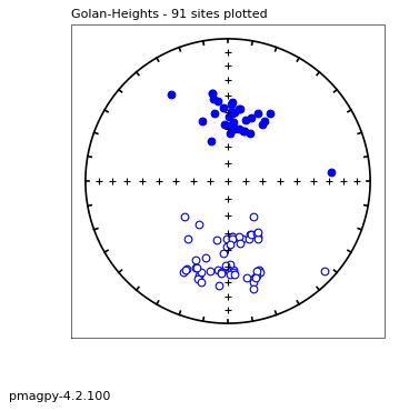
../../_images/2022_MagIC_database_and_open_science_19_2.png

Figure 3: Equal area plot of the directions from the downloaded data set. North is at the top of the diagram and vertical is in the center. Solid (open) symbols are downward (upward) directed. There are two sets of directions, one pointed north and down and one pointed south and up.

Saving plots#

to save the plots, set save_plots to True and your preferred format using the argument, fmt.
you can download the resulting png file (or find it in your project directory if running locally).

ipmag.eqarea_magic(dir_path=dir_path,save_plots=True,fmt='png')

91  sites records read in
1  saved in  /Users/ltauxe/PmagPy/MagIC_for_earthcube/all_Golan-Heights_g_eqarea.png

(True,
 ['/Users/ltauxe/PmagPy/MagIC_for_earthcube/all_Golan-Heights_g_eqarea.png'])

Are the two sets of directions antipodal?#

One can see in Figure 3 that there are two sets of directions, one to the north and down (as expected for the latitude of the Golan Heights in Israel and one directed to the south and up (as expected for a reverse field in Israel). So, are the two sets of directions antipodal? PmagPy has code to test this hypothesis. Here we will use the bootstrap reversal test (see opensource textbook Essentials of Paleomagnetism at: https://earthref.org/MagIC/books/Tauxe/Essentials/) to see if the two sets are antipodal.

help(ipmag.reversal_test_bootstrap)

Help on function reversal_test_bootstrap in module pmagpy.ipmag:

reversal_test_bootstrap(dec=None, inc=None, di_block=None, plot_stereo=False, save=False, save_folder='.', fmt='svg')
    Conduct a reversal test using bootstrap statistics (Tauxe, 2010) to
    determine whether two populations of directions could be from an antipodal
    common mean.
    
    Parameters
    ----------
    dec: list of declinations
    inc: list of inclinations
        or
    di_block: a nested list of [dec,inc]
        A di_block can be provided in which case it will be used instead of
        dec, inc lists.
    
    plot_stereo : before plotting the CDFs, plot stereonet with the
        bidirectionally separated data (default is False)
    save : boolean argument to save plots (default is False)
    save_folder : directory where plots will be saved (default is current directory, '.')
    fmt : format of saved figures (default is 'svg')
    
    Returns
    -------
    plots : Plots of the cumulative distribution of Cartesian components are
        shown as is an equal area plot if plot_stereo = True
    
    Examples
    --------
    Populations of roughly antipodal directions are developed here using
    ``ipmag.fishrot``. These directions are combined into a single di_block
    given that the function determines the principal component and splits the
    data accordingly by polarity.
    
    >>> directions_n = ipmag.fishrot(k=20, n=30, dec=5, inc=-60)
    >>> directions_r = ipmag.fishrot(k=35, n=25, dec=182, inc=57)
    >>> directions = directions_n + directions_r
    >>> ipmag.reversal_test_bootstrap(di_block=directions, plot_stereo = True)
    
    Data can also be input to the function as separate lists of dec and inc.
    In this example, the di_block from above is split into lists of dec and inc
    which are then used in the function:
    
    >>> direction_dec, direction_inc, direction_moment = ipmag.unpack_di_block(directions)
    >>> ipmag.reversal_test_bootstrap(dec=direction_dec,inc=direction_inc, plot_stereo = True)

We already read in the directional data into a Pandas DataFrame df, so lets pick out the lists of declinations and inclinations and feed them into ipmag.reversal_test_bootstrap. This program first converts one of the sets of directions to their antipodes (by adding 180\(^{\circ}\) to the declinations and taking the opposition of the inclinations. It then calculates the mean directions from 1000 “pseudosamples” of the two data sets and plots the resulting means (converted to their cartesian coordinates) as cumulative distributions. If there is overlap in all three components, then the data sets are likely antipodal.

Consulting the MagIC data model page for the sites data table, we see that the desired column headers are ‘dir_dec’ and ‘dir_inc’ for declination and inclination. So we can make arrays (or lists) of those and feed them into our reversals test as follows:

decs=df['dir_dec'].values
incs=df['dir_inc'].values
ipmag.reversal_test_bootstrap(dec=decs,inc=incs)

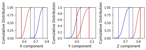
../../_images/2022_MagIC_database_and_open_science_26_0.png

Here we see that the X and Z components are NOT antipodal as the 95% confidence limits (vertical lines) of the bootstrapped means do not overlap. So this data set fails the reversals test.

Map of equivalent VGPs#

We can explore the data set further by converting the directions to their equivalent virtual geomagnetic poles (VGPs). The transformation and the plot is done for is by the PmagPy function ipmag.vgpmap_magic().

help(ipmag.vgpmap_magic)

Help on function vgpmap_magic in module pmagpy.ipmag:

vgpmap_magic(dir_path='.', results_file='sites.txt', crd='', sym='ro', size=8, rsym='g^', rsize=8, fmt='pdf', res='c', proj='ortho', flip=False, anti=False, fancy=False, ell=False, ages=False, lat_0=0, lon_0=0, save_plots=True, interactive=False, contribution=None, image_records=False)
    makes a map of vgps and a95/dp,dm for site means in a sites table
    
    Parameters
    ----------
    dir_path : str, default "."
        input directory path
    results_file : str, default "sites.txt"
        name of MagIC format sites file
    crd : str, default ""
       coordinate system [g, t] (geographic, tilt_corrected)
    sym : str, default "ro"
        symbol color and shape, default red circles
        (see matplotlib documentation for more color/shape options)
    size : int, default 8
        symbol size
    rsym : str, default "g^"
        symbol for plotting reverse poles
        (see matplotlib documentation for more color/shape options)
    rsize : int, default 8
        symbol size for reverse poles
    fmt : str, default "pdf"
        format for figures, ["svg", "jpg", "pdf", "png"]
    res : str, default "c"
        resolution [c, l, i, h] (crude, low, intermediate, high)
    proj : str, default "ortho"
        ortho = orthographic
        lcc = lambert conformal
        moll = molweide
        merc = mercator
    flip : bool, default False
        if True, flip reverse poles to normal antipode
    anti : bool, default False
        if True, plot antipodes for each pole
    fancy : bool, default False
        if True, plot topography (not yet implemented)
    ell : bool, default False
        if True, plot ellipses
    ages : bool, default False
        if True, plot ages
    lat_0 : float, default 0.
        eyeball latitude
    lon_0 : float, default 0.
        eyeball longitude
    save_plots : bool, default True
        if True, create and save all requested plots
    interactive : bool, default False
       if True, interactively plot and display
        (this is best used on the command line only)
    image_records : bool, default False
        if True, return a list of created images
    
    Returns
    ---------
    if image_records == False:
        type - Tuple : (True or False indicating if conversion was successful, file name(s) written)
    if image_records == True:
       Tuple : (True or False indicating if conversion was successful, output file name written, list of image recs)

ipmag.vgpmap_magic(dir_path=dir_path,size=50,flip=True,save_plots=False,lat_0=60,rsym='b^',rsize=50,fmt='png')

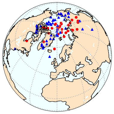
../../_images/2022_MagIC_database_and_open_science_30_0.png

Figure 4: Orthographic projection of virtual geomagnetic poles calculated from directional data of Behar et al. (2019). Red dots are for the normal poles and blue squares are the antipodes of the reverse poles.

By setting the argument flip to True, we can plot the normal (red dots) and the reverse (blue triangles) poles on the same projection. Behar et al. (2019) attributed the difference in mean directions to a tectonic tilting event that offset the two sets.

Next steps:#

Try out other Jupyter notebooks within the PmagPy software distribution to learn the full functionality of the package either by installing PmagPy on a personal computer (see https://earthref.org/PmagPy/cookbook/) or run PmagPy notebooks without installation through the website: https://jupyterhub.earthref.org. You will have to create a username using an ORCID which will allow you to upload your own data, or download data from the MagIC website, create plots and save them and preserve your work in your own permanent space. Using the FIESTA API, datasets can be uploaded to a Private Workspace in the MagIC database and published when your manuscript gets accepted.
Become a PmagPy developer!

References#

Behar, N., Shaar, R., Tauxe, L., Asefaw, H., Ebert, Y., Heimann, A., Koppers, A.A.P., and Ron, H. (2019), Paleomagnetic study of the Plio-Pleistocene Golan Heights volcanic field, Israel: confirmation of the GAD field hypothesis, Geophys., Geochem. Geosyst., 20, https://dx.doi.org/10.1029/2019GC008479.
MagIC website: https://earthref.org/MagIC
EarthRef FIESTA API: https://api.earthref.org
Textbook for paleomagnetism: https://earthref.org/MagIC/books/Tauxe/Essentials/
PmagPy installation instructions: https://earthref.org/PmagPy/cookbook/
Course in Python for Earth Science Students: https://github.com/ltauxe/Python-for-Earth-Science-Students
PmagPy citation: Tauxe, L., R. Shaar, L. Jonestrask, N. L. Swanson-Hysell, R. Minnett, A. A. P. Koppers, C. G. Constable, N. Jarboe, K. Gaastra, and L. Fairchild (2016), PmagPy: Software package for paleomagnetic data analysis and a bridge to the Magnetics Information Consortium (MagIC) Database, Geochem. Geophys. Geosyst., 17, https://doi.org/10.1002/2016GC006307.

EarthCube 2022 Call for Notebooks

Jupyter Notebooks as a bridge to the MagIC Database and Open Science

Contents